Constructs and draws a zigzag expanded navigation plot for a graphical exploratory analysis of a path of variables. The result is an alternating sequence of one-dimensional (1d) and two-dimensional (2d) plots laid out in a zigzag-like structure so that each consecutive pair of 2d plots has one of its variates (or coordinates) in common with that of the 1d plot appearing between them.
Usage
zenplot(x, turns = NULL,
        first1d = TRUE, last1d = TRUE,
        n2dcols = c("letter", "square", "A4", "golden", "legal"),
        n2dplots = NULL,
        plot1d = c("label", "points", "jitter", "density", "boxplot", "hist",
                   "rug", "arrow", "rect", "lines", "layout"),
        plot2d = c("points", "density", "axes", "label", "arrow", "rect", "layout"),
        zargs = c(x = TRUE, turns = TRUE, orientations = TRUE,
                  vars = TRUE, num = TRUE, lim = TRUE, labs = TRUE,
                  width1d = TRUE, width2d = TRUE,
                  ispace = match.arg(pkg) != "graphics"),
        lim = c("individual", "groupwise", "global"),
        labs = list(group = "G", var = "V", sep = ", ", group2d = FALSE),
        pkg = c("graphics", "grid", "loon"),
        method = c("tidy", "double.zigzag", "single.zigzag", "rectangular"),
        width1d = if(is.null(plot1d)) 0.5 else 1,
        width2d = 10,
        ospace = if(pkg == "loon") 0 else 0.02,
        ispace = if(pkg == "graphics") 0 else 0.037,
        draw = TRUE,
        ...)
Arguments
- x
A data object of "standard forms", being a
vector, or amatrix, or adata.frame, or alistof any of these. In the case of a list, the components ofxare interpreted as groups of data which are visually separated by a two-dimensional (group) plot.- turns
A
charactervector (of length two times the number of variables to be plotted minus 1) consisting of"d","u","r"or"l"indicating the turns out of the current plot position; ifNULL, theturnsare constructed (ifxis of the "standard form" described above).- first1d
A
logicalindicating whether the first one-dimensional plot is included.- last1d
A
logicalindicating whether the last one-dimensional plot is included.- n2dcols
number of columns of 2d plots (\(\ge 1\)) or one of
"letter","square","A4","golden"or"legal"in which case a similar layout is constructed. Note thatn2dcolsis ignored if!is.null(turns).- n2dplots
The number of 2d plots.
- plot1d
A
functionto use to return a one-dimensional plot constructed with packagepkg. Alternatively, acharacterstring of an existing function. For the defaults provided, the corresponding functions are obtained when appending_1d_graphics,_1d_gridor_1d_loondepending on whichpkgis used.If
plot1d = NULL, then no 1d plot is produced in thezenplot.- plot2d
A
functionreturning a two-dimensional plot constructed with packagepkg. Alternatively, acharacterstring of an existing function. For the defaults provided, the corresponding functions are obtained when appending_2d_graphics,_2d_gridor_2d_loondepending on whichpkgis used.As for
plot1d,plot2domits 2d plots ifplot2d = NULL.- zargs
A fully named
logicalvectorindicating whether the respective arguments are (possibly) passed toplot1d()andplot2d()(if the latter contain the formal argumentzargs, which they typically do/should, but see below for an example in which they do not).zargscan maximally contain all variables as given in the default. If one of those variables does not appear inzargs, it is treated asTRUEand the corresponding arguments are passed on toplot1dandplot2d. If one of them is set toFALSE, the argument is not passed on.- lim
(x-/y-)axis limits. This can be a
characterstring or anumeric(2).If
lim = "groupwise"andxdoes not contain groups, the behaviour is equivalent tolim = "global".- labs
The plot labels to be used; see the argument
labsofburst()for the exact specification.labscan, in general, be anything as long asplot1dandplot2dknow how to deal with it.- pkg
The R package used for plotting (depends on how the functions
plot1dandplot2dwere constructed; the user is responsible for choosing the appropriate package among the supported ones).- method
The type of zigzag plot (a
character).Available are:
tidy:more tidied-up
double.zigzag(slightly more compact placement of plots towards the end).double.zigzag:zigzag plot in the form of a flipped “S”. Along this path, the plots are placed in the form of an “S” which is rotated counterclockwise by 90 degrees.
single.zigzag:zigzag plot in the form of a flipped “S”.
rectangular:plots that fill the page from left to right and top to bottom. This is useful (and most compact) for plots that do not share an axis.
Note that
methodis ignored ifturnsare provided.- width1d
A graphical parameter > 0 giving the width of 1d plots.
- width2d
A graphical parameter > 0 giving the height of 2d plots.
- ospace
The outer space around the zenplot. A vector of length four (bottom, left, top, right), or one whose values are repeated to be of length four, which gives the outer space between the device region and the inner plot region around the zenplot.
Values should be in \([0,1]\) when
pkgis"graphics"or"grid", and as number of pixels whenpkgis"loon".- ispace
The inner space in \([0,1]\) between the each figure region and the region of the (1d/2d) plot it contains. Again, a vector of length four (bottom, left, top, right) or a shorter one whose values are repeated to produce a vector of length four.
- draw
A
logicalindicating whether a thezenplotis immediately displayed (the default) or not.- ...
arguments passed to the drawing functions for both
plot1dandplot2d. If you need to pass certain arguments only to one of them, say,plot2d, consider providing your ownplot2d; see the examples below.
Value
(besides plotting) invisibly returns a list having additional classnames marking it as a zenplot and a zenPkg object (with Pkg being one of Graphics, Grid, or Loon, so as to identify the package used to construct the plot).
As a list it contains at least
the path and layout (see unfold for details).
Depending on the graphics package pkg used, the returned list
includes additional components. For pkg = "grid",
this will be the whole plot as a grob (grid object).
For pkg = "loon", this will be the whole plot as a
loon plot object as
well as the toplevel tk object in which the plot appears.
See also
All provided default plot1d and plot2d functions.
extract_1d() and extract_2d()
for how zargs can be split up into a list of columns and corresponding
group and variable information.
burst() for how x can be split up into all sorts of
information useful for plotting (see our default plot1d and plot2d).
vport() for how to construct a viewport for
(our default) grid (plot1d and plot2d) functions.
extract_pairs(), connect_pairs(),
group() and zenpath() for
(zen)path-related functions.
The various vignettes for additional examples.
Other creating zenplots:
unfold()
Examples
### Basics #####################################################################
## Generate some data
n <- 1000 # sample size
d <- 20 # dimension
set.seed(271) # set seed (for reproducibility)
x <- matrix(rnorm(n * d), ncol = d) # i.i.d. N(0,1) data
## A basic zenplot
res <- zenplot(x)
 uf <- unfold(nfaces = d - 1)
## `res` and `uf` is not identical as `res` has specific
## class attributes.
for(name in names(uf)) {
stopifnot(identical(res[[name]], uf[[name]]))
}
## => The return value of zenplot() is the underlying unfold()
## Some missing data
z <- x
z[seq_len(n-10), 5] <- NA # all NA except 10 points
zenplot(z)
uf <- unfold(nfaces = d - 1)
## `res` and `uf` is not identical as `res` has specific
## class attributes.
for(name in names(uf)) {
stopifnot(identical(res[[name]], uf[[name]]))
}
## => The return value of zenplot() is the underlying unfold()
## Some missing data
z <- x
z[seq_len(n-10), 5] <- NA # all NA except 10 points
zenplot(z)
 ## Another column with fully missing data (use arrows)
## Note: This could be more 'compactified', but is technically
## more involved
z[, 6] <- NA # all NA
zenplot(z)
## Another column with fully missing data (use arrows)
## Note: This could be more 'compactified', but is technically
## more involved
z[, 6] <- NA # all NA
zenplot(z)
 ## Lists of vectors, matrices and data frames as arguments (=> groups of data)
## Only two vectors
z <- list(x[,1], x[,2])
zenplot(z)
## Lists of vectors, matrices and data frames as arguments (=> groups of data)
## Only two vectors
z <- list(x[,1], x[,2])
zenplot(z)
 ## A matrix and a vector
z <- list(x[,1:2], x[,3])
zenplot(z)
## A matrix and a vector
z <- list(x[,1:2], x[,3])
zenplot(z)
 ## A matrix, NA column and a vector
z <- list(x[,1:2], NA, x[,3])
zenplot(z)
## A matrix, NA column and a vector
z <- list(x[,1:2], NA, x[,3])
zenplot(z)
 z <- list(x[,1:2], cbind(NA, NA), x[,3])
zenplot(z)
z <- list(x[,1:2], cbind(NA, NA), x[,3])
zenplot(z)
 z <- list(x[,1:2], 1:10, x[,3])
zenplot(z)
z <- list(x[,1:2], 1:10, x[,3])
zenplot(z)
 ## Without labels or with different labels
z <- list(A = x[,1:2], B = cbind(NA, NA), C = x[,3])
zenplot(z, labs = NULL) # without any labels
## Without labels or with different labels
z <- list(A = x[,1:2], B = cbind(NA, NA), C = x[,3])
zenplot(z, labs = NULL) # without any labels
 # without group labels
zenplot(z, labs = list(group = NULL, group2d = TRUE))
# without group labels
zenplot(z, labs = list(group = NULL, group2d = TRUE))
 # without group labels unless groups change
zenplot(z, labs = list(group = NULL))
# without group labels unless groups change
zenplot(z, labs = list(group = NULL))
 # without variable labels
zenplot(z, labs = list(var = NULL))
# without variable labels
zenplot(z, labs = list(var = NULL))
 # change default labels
zenplot(z, labs = list(var = "Variable ", sep = " - "))
# change default labels
zenplot(z, labs = list(var = "Variable ", sep = " - "))
 ## Example with a factor
zenplot(iris)
## Example with a factor
zenplot(iris)
 zenplot(iris, lim = "global") # global scaling of axis
 # acts as 'global' here (no groups in the data)
zenplot(iris, lim = "groupwise")
### More sophisticated examples ################################################
## Note: The third component (data.frame) naturally has default labels.
## zenplot() uses these labels and prepends a default group label.
z <- list(x[,1:5], x[1:10, 6:7], NA,
data.frame(x[seq_len(round(n/5)), 8:19]), cbind(NA, NA), x[1:10, 20])
# change the group label (var and sep are defaults)
zenplot(z, labs = list(group = "Group "))
# acts as 'global' here (no groups in the data)
zenplot(iris, lim = "groupwise")
### More sophisticated examples ################################################
## Note: The third component (data.frame) naturally has default labels.
## zenplot() uses these labels and prepends a default group label.
z <- list(x[,1:5], x[1:10, 6:7], NA,
data.frame(x[seq_len(round(n/5)), 8:19]), cbind(NA, NA), x[1:10, 20])
# change the group label (var and sep are defaults)
zenplot(z, labs = list(group = "Group "))
 ## Alternatively, give z labels
# give group names
names(z) <- paste("Group", LETTERS[seq_len(length(z))])
zenplot(z) # uses given group names
## Alternatively, give z labels
# give group names
names(z) <- paste("Group", LETTERS[seq_len(length(z))])
zenplot(z) # uses given group names
 ## Now let's change the variable labels
z. <- lapply(z, function(z.) {
if(!is.matrix(z.)) z. <- as.matrix(z.)
colnames(z.) <- paste("Var.", seq_len(ncol(z.)))
z.
}
)
zenplot(z.)
## Now let's change the variable labels
z. <- lapply(z, function(z.) {
if(!is.matrix(z.)) z. <- as.matrix(z.)
colnames(z.) <- paste("Var.", seq_len(ncol(z.)))
z.
}
)
zenplot(z.)
 ### A dynamic plot based on 'loon'
# (if installed and R compiled with tcl support)
if (FALSE) { # \dontrun{
if (requireNamespace("loon", quietly = TRUE))
zenplot(x, pkg = "loon")
} # }
### Providing your own turns ###################################################
## A basic example
turns <- c("l","d","d","r","r","d","d","r","r",
"u","u","r","r","u","u","l","l",
"u","u","l","l","u","u","l","l",
"d","d","l","l","d","d","l","l",
"d","d","r","r","d","d")
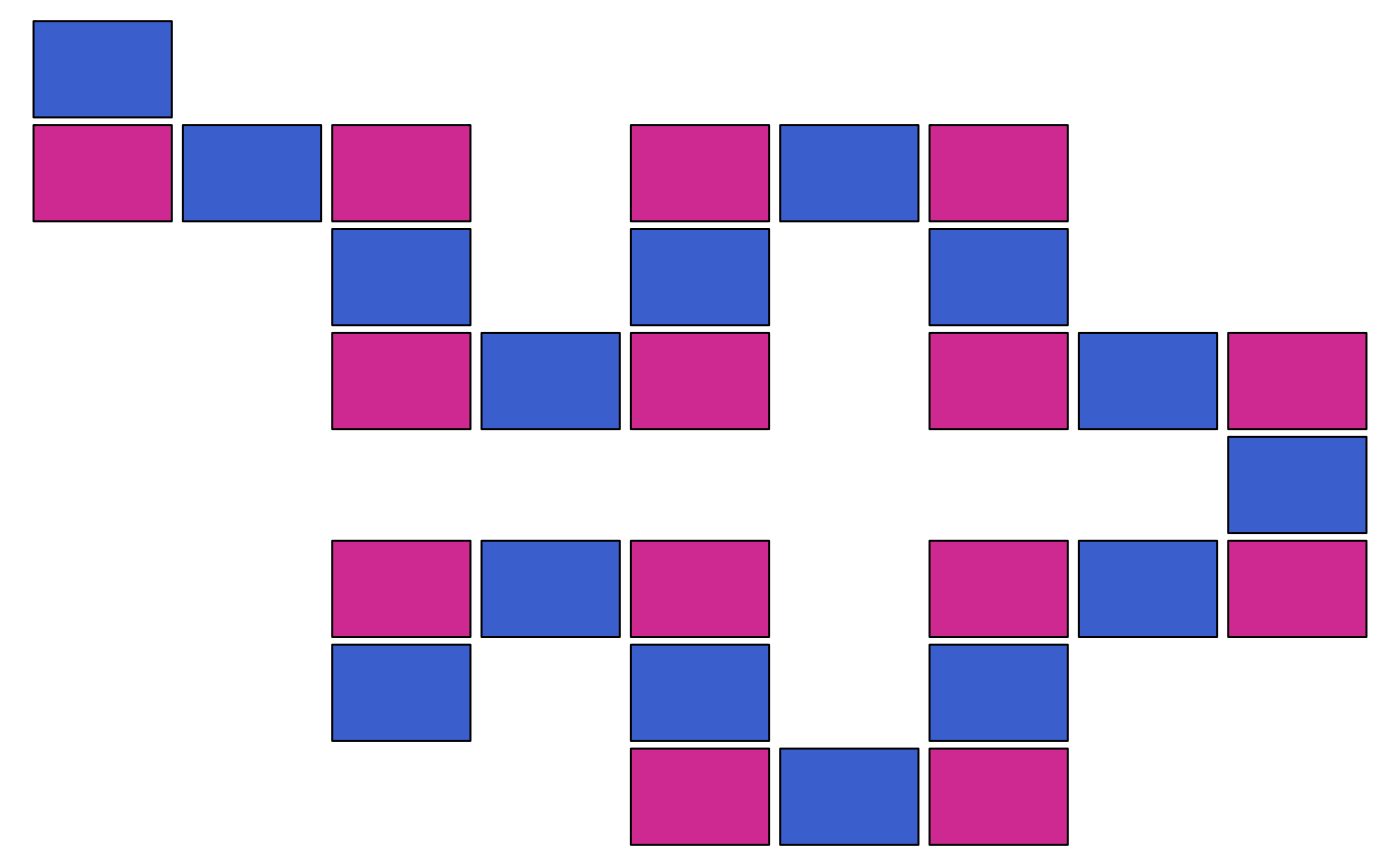
# layout of plot regions
# => The tiles stick together as ispace = 0.
zenplot(x, plot1d = "layout", plot2d = "layout", turns = turns)
### A dynamic plot based on 'loon'
# (if installed and R compiled with tcl support)
if (FALSE) { # \dontrun{
if (requireNamespace("loon", quietly = TRUE))
zenplot(x, pkg = "loon")
} # }
### Providing your own turns ###################################################
## A basic example
turns <- c("l","d","d","r","r","d","d","r","r",
"u","u","r","r","u","u","l","l",
"u","u","l","l","u","u","l","l",
"d","d","l","l","d","d","l","l",
"d","d","r","r","d","d")
# layout of plot regions
# => The tiles stick together as ispace = 0.
zenplot(x, plot1d = "layout", plot2d = "layout", turns = turns)
 # layout of plot regions with grid
# => Here the tiles show the small (default) ispace
zenplot(x, plot1d = "layout", plot2d = "layout",
turns = turns,
pkg = "grid")
# layout of plot regions with grid
# => Here the tiles show the small (default) ispace
zenplot(x, plot1d = "layout", plot2d = "layout",
turns = turns,
pkg = "grid")
 ## Another example (with own turns and groups)
zenplot(list(x[,1:3], x[,4:7]), plot1d = "arrow", plot2d = "rect",
turns = c("d", "r", "r", "r", "r", "d",
"d", "l", "l", "l", "l", "l"), last1d = FALSE)
## Another example (with own turns and groups)
zenplot(list(x[,1:3], x[,4:7]), plot1d = "arrow", plot2d = "rect",
turns = c("d", "r", "r", "r", "r", "d",
"d", "l", "l", "l", "l", "l"), last1d = FALSE)
 ### Providing your own plot1d() or plot2d() ####################################
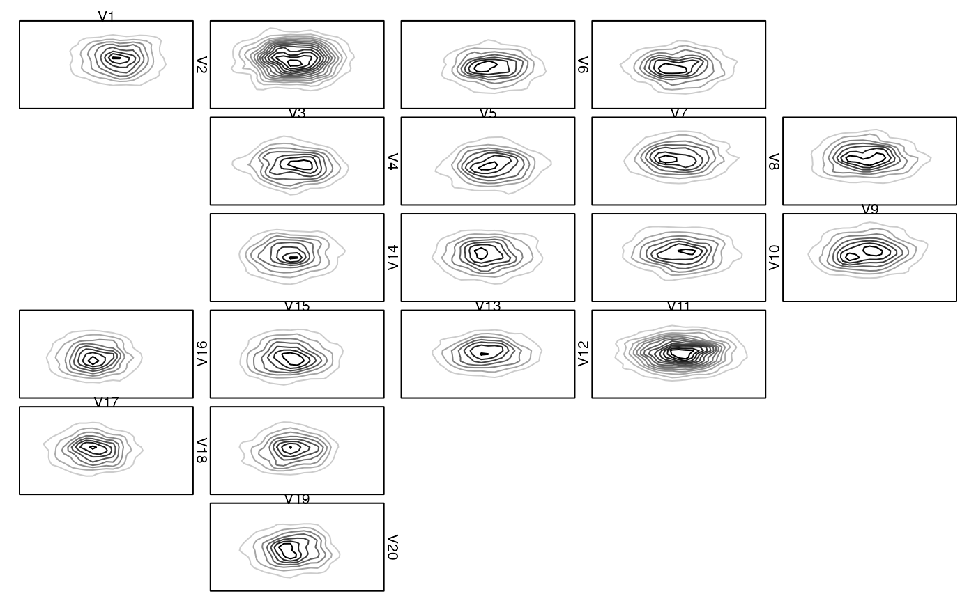
## Creating a box
zenplot(x, plot1d = "label", plot2d = function(zargs)
density_2d_graphics(zargs, box = TRUE))
### Providing your own plot1d() or plot2d() ####################################
## Creating a box
zenplot(x, plot1d = "label", plot2d = function(zargs)
density_2d_graphics(zargs, box = TRUE))
 ## With grid
# (grid is in Imports; call fully-qualified to avoid library())
# \donttest{
zenplot(x, plot1d = "label", plot2d = function(zargs)
density_2d_grid(zargs, box = TRUE), pkg = "grid")
## With grid
# (grid is in Imports; call fully-qualified to avoid library())
# \donttest{
zenplot(x, plot1d = "label", plot2d = function(zargs)
density_2d_grid(zargs, box = TRUE), pkg = "grid")
 # }
## An example with width1d = width2d and where no zargs are passed on.
## Note: This could have also been done with
## 'rect_2d_graphics(zargs, col = ...)'
## as plot1d and plot2d.
myrect <- function(...) {
plot(NA, type = "n", ann = FALSE, axes = FALSE,
xlim = 0:1, ylim = 0:1)
rect(xleft = 0, ybottom = 0, xright = 1, ytop = 1, ...)
}
zenplot(matrix(0, ncol = 15),
n2dcol = "square", width1d = 10, width2d = 10,
plot1d = function(...) myrect(col = "royalblue3"),
plot2d = function(...) myrect(col = "maroon3"))
# }
## An example with width1d = width2d and where no zargs are passed on.
## Note: This could have also been done with
## 'rect_2d_graphics(zargs, col = ...)'
## as plot1d and plot2d.
myrect <- function(...) {
plot(NA, type = "n", ann = FALSE, axes = FALSE,
xlim = 0:1, ylim = 0:1)
rect(xleft = 0, ybottom = 0, xright = 1, ytop = 1, ...)
}
zenplot(matrix(0, ncol = 15),
n2dcol = "square", width1d = 10, width2d = 10,
plot1d = function(...) myrect(col = "royalblue3"),
plot2d = function(...) myrect(col = "maroon3"))
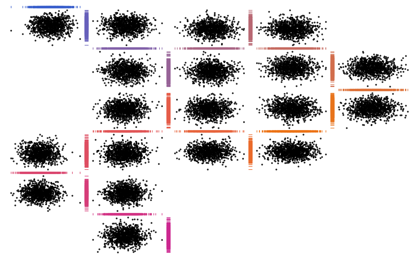
 ## Colorized rugs as plot1d()
basecol <- c("royalblue3", "darkorange2", "maroon3")
palette <- grDevices::colorRampPalette(basecol, space = "Lab")
cols <- palette(d) # different color for each 1d plot
zenplot(x, plot1d = function(zargs) {
rug_1d_graphics(zargs, col = cols[(zargs$num+1)/2])
}
)
## Colorized rugs as plot1d()
basecol <- c("royalblue3", "darkorange2", "maroon3")
palette <- grDevices::colorRampPalette(basecol, space = "Lab")
cols <- palette(d) # different color for each 1d plot
zenplot(x, plot1d = function(zargs) {
rug_1d_graphics(zargs, col = cols[(zargs$num+1)/2])
}
)
 ## With grid (no library(), fully qualify)
# \donttest{
zenplot(x, pkg = "grid",
plot1d = function(zargs)
rug_1d_grid(zargs, col = cols[(zargs$num+1)/2]))
## With grid (no library(), fully qualify)
# \donttest{
zenplot(x, pkg = "grid",
plot1d = function(zargs)
rug_1d_grid(zargs, col = cols[(zargs$num+1)/2]))
 # }
## Rectangles with labels as plot2d() (shows how to overlay plots)
## With graphics
zenplot(x, plot1d = "arrow", plot2d = function(zargs) {
rect_2d_graphics(zargs)
label_2d_graphics(zargs, add = TRUE)
})
# }
## Rectangles with labels as plot2d() (shows how to overlay plots)
## With graphics
zenplot(x, plot1d = "arrow", plot2d = function(zargs) {
rect_2d_graphics(zargs)
label_2d_graphics(zargs, add = TRUE)
})
 ## With grid (no library(), fully qualify grid helpers)
# \donttest{
zenplot(x, pkg = "grid", plot1d = "arrow", plot2d = function(zargs)
grid::gTree(children = grid::gList(rect_2d_grid(zargs),
label_2d_grid(zargs))))
## With grid (no library(), fully qualify grid helpers)
# \donttest{
zenplot(x, pkg = "grid", plot1d = "arrow", plot2d = function(zargs)
grid::gTree(children = grid::gList(rect_2d_grid(zargs),
label_2d_grid(zargs))))
 # }
## Rectangles with labels outside the 2d plotting region as plot2d()
## With graphics
zenplot(x, plot1d = "arrow", plot2d = function(zargs) {
rect_2d_graphics(zargs)
label_2d_graphics(zargs, add = TRUE, xpd = NA, srt = 90,
loc = c(1.04, 0), adj = c(0,1), cex = 0.7)
})
# }
## Rectangles with labels outside the 2d plotting region as plot2d()
## With graphics
zenplot(x, plot1d = "arrow", plot2d = function(zargs) {
rect_2d_graphics(zargs)
label_2d_graphics(zargs, add = TRUE, xpd = NA, srt = 90,
loc = c(1.04, 0), adj = c(0,1), cex = 0.7)
})
 ## With grid (no library(), fully qualify)
# \donttest{
zenplot(x, pkg = "grid", plot1d = "arrow", plot2d = function(zargs)
grid::gTree(children =
grid::gList(rect_2d_grid(zargs),
label_2d_grid(zargs, loc = c(1.04, 0),
just = c("left", "top"),
rot = 90, cex = 0.45))))
## With grid (no library(), fully qualify)
# \donttest{
zenplot(x, pkg = "grid", plot1d = "arrow", plot2d = function(zargs)
grid::gTree(children =
grid::gList(rect_2d_grid(zargs),
label_2d_grid(zargs, loc = c(1.04, 0),
just = c("left", "top"),
rot = 90, cex = 0.45))))
 # }
## 2d density with points, 1d arrows and labels
zenplot(x,
plot1d = function(zargs) {
rect_1d_graphics(zargs)
arrow_1d_graphics(zargs,
add = TRUE,
loc = c(0.2, 0.5))
label_1d_graphics(zargs,
add = TRUE,
loc = c(0.8, 0.5))
},
plot2d = function(zargs) {
points_2d_graphics(zargs,
col =
grDevices::adjustcolor("black",
alpha.f = 0.4))
density_2d_graphics(zargs, add = TRUE)
}
)
# }
## 2d density with points, 1d arrows and labels
zenplot(x,
plot1d = function(zargs) {
rect_1d_graphics(zargs)
arrow_1d_graphics(zargs,
add = TRUE,
loc = c(0.2, 0.5))
label_1d_graphics(zargs,
add = TRUE,
loc = c(0.8, 0.5))
},
plot2d = function(zargs) {
points_2d_graphics(zargs,
col =
grDevices::adjustcolor("black",
alpha.f = 0.4))
density_2d_graphics(zargs, add = TRUE)
}
)
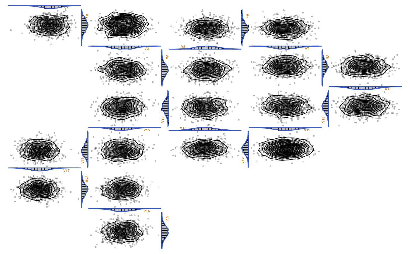
 ## 2d density with labels, 1d histogram with density and label
zenplot(x,
plot1d = function(zargs) {
hist_1d_graphics(zargs)
density_1d_graphics(zargs, add = TRUE,
border = "royalblue3",
lwd = 1.4)
label_1d_graphics(zargs, add = TRUE,
loc = c(0.2, 0.8),
cex = 0.6, font = 2,
col = "darkorange2")
},
plot2d = function(zargs) {
density_2d_graphics(zargs)
points_2d_graphics(zargs, add = TRUE,
col =
grDevices::adjustcolor("black",
alpha.f = 0.3))
}
)
## 2d density with labels, 1d histogram with density and label
zenplot(x,
plot1d = function(zargs) {
hist_1d_graphics(zargs)
density_1d_graphics(zargs, add = TRUE,
border = "royalblue3",
lwd = 1.4)
label_1d_graphics(zargs, add = TRUE,
loc = c(0.2, 0.8),
cex = 0.6, font = 2,
col = "darkorange2")
},
plot2d = function(zargs) {
density_2d_graphics(zargs)
points_2d_graphics(zargs, add = TRUE,
col =
grDevices::adjustcolor("black",
alpha.f = 0.3))
}
)
 ### More sophisticated examples ################################################
### Example: Overlaying histograms with densities (the *proper* way)
# \donttest{
## Define proper 1d plot for overlaying histograms with densities
hist_with_density_1d <- function(zargs)
{
num <- zargs$num
turn.out <- zargs$turns[num]
horizontal <- turn.out == "d" || turn.out == "u"
ii <- plot_indices(zargs)
label <- paste0("V", ii[1])
srt <- if(horizontal) 0 else if(turn.out == "r") -90 else 90
x <- zargs$x[,ii[1]]
lim <- range(x)
breaks <- seq(from = lim[1], to = lim[2], length.out = 21)
binInfo <- hist(x, breaks = breaks, plot = FALSE)
binBoundaries <- binInfo$breaks
widths <- diff(binBoundaries)
heights <- binInfo$density
dens <- density(x)
xvals <- dens$x
keepers <- (min(x) <= xvals) & (xvals <= max(x))
x. <- xvals[keepers]
y. <- dens$y[keepers]
if(turn.out == "d" || turn.out == "l") {
heights <- -heights; y. <- -y.
}
if(horizontal) {
xlim <- lim; xlim.bp <- xlim - xlim[1]
ylim <- range(0, heights, y.); ylim.bp <- ylim
x <- c(xlim[1], x., xlim[2]) - xlim[1]; y <- c(0, y., 0)
} else {
xlim <- range(0, heights, y.); xlim.bp <- xlim
ylim <- lim; ylim.bp <- ylim - ylim[1]
x <- c(0, y., 0); y <- c(xlim[1], x., xlim[2]) - ylim[1]
}
loc <- c(0.1, 0.6)
if(turn.out == "d") loc <- 1 - loc
if(turn.out == "r") { loc <- rev(loc); loc[2] <- 1 - loc[2] }
if(turn.out == "l") { loc <- rev(loc); loc[1] <- 1 - loc[1] }
barplot(heights, width = widths, xlim = xlim.bp, ylim = ylim.bp,
space = 0, horiz = !horizontal,
main = "", xlab = "", axes = FALSE)
polygon(x = x, y = y, border = "royalblue3", lwd = 1.4)
opar <- par(usr = c(0, 1, 0, 1)); on.exit(par(opar))
text(x = loc[1], y = loc[2], labels = label,
cex = 0.7, srt = srt, font = 2,
col = "darkorange2")
}
zenplot(x,
plot1d = "hist_with_density_1d",
plot2d = function(zargs) {
density_2d_graphics(zargs)
points_2d_graphics(zargs, add = TRUE,
col = grDevices::adjustcolor("black",
alpha.f = 0.3))
})
#> Error in zenplot(x, plot1d = "hist_with_density_1d", plot2d = function(zargs) { density_2d_graphics(zargs) points_2d_graphics(zargs, add = TRUE, col = grDevices::adjustcolor("black", alpha.f = 0.3))}): Function provided as argument 'plot1d' does not exist.
# }
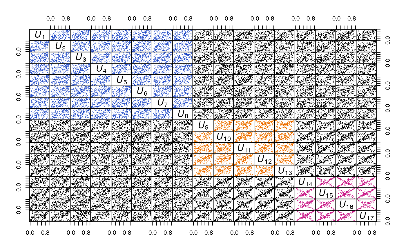
### Example: A path through pairs of a grouped t copula sample
# \donttest{
d. <- c(8, 5, 4); d <- sum(d.); nu <- rep(c(12, 1, 0.25), times = d.)
n <- 500; set.seed(271)
Z <- matrix(rnorm(n * d), ncol = n)
P <- matrix(0.5, nrow = d, ncol = d); diag(P) <- 1
L <- t(chol(P)); Y <- t(L %*% Z)
U. <- runif(n)
W <- sapply(nu, function(nu.) 1/qgamma(U., shape = nu./2, rate = nu./2))
X <- sqrt(W) * Y
U <- sapply(1:d, function(j) pt(X[,j], df = nu[j]))
cols <- matrix("black", nrow = d, ncol = d)
start <- c(1, cumsum(head(d., n = -1))+1)
end <- cumsum(d.)
for(j in seq_along(d.)) cols[start[j]:end[j], start[j]:end[j]] <- basecol[j]
diag(cols) <- NA
cols <- as.vector(cols); cols <- cols[!is.na(cols)]
count <- 0
my_panel <- function(x, y, ...) {
count <<- count + 1
points(x, y, pch = ".", col = cols[count])
}
pairs(U, panel = my_panel, gap = 0,
labels = as.expression(sapply(1:d,
function(j) bquote(italic(U[.(j)])))))
### More sophisticated examples ################################################
### Example: Overlaying histograms with densities (the *proper* way)
# \donttest{
## Define proper 1d plot for overlaying histograms with densities
hist_with_density_1d <- function(zargs)
{
num <- zargs$num
turn.out <- zargs$turns[num]
horizontal <- turn.out == "d" || turn.out == "u"
ii <- plot_indices(zargs)
label <- paste0("V", ii[1])
srt <- if(horizontal) 0 else if(turn.out == "r") -90 else 90
x <- zargs$x[,ii[1]]
lim <- range(x)
breaks <- seq(from = lim[1], to = lim[2], length.out = 21)
binInfo <- hist(x, breaks = breaks, plot = FALSE)
binBoundaries <- binInfo$breaks
widths <- diff(binBoundaries)
heights <- binInfo$density
dens <- density(x)
xvals <- dens$x
keepers <- (min(x) <= xvals) & (xvals <= max(x))
x. <- xvals[keepers]
y. <- dens$y[keepers]
if(turn.out == "d" || turn.out == "l") {
heights <- -heights; y. <- -y.
}
if(horizontal) {
xlim <- lim; xlim.bp <- xlim - xlim[1]
ylim <- range(0, heights, y.); ylim.bp <- ylim
x <- c(xlim[1], x., xlim[2]) - xlim[1]; y <- c(0, y., 0)
} else {
xlim <- range(0, heights, y.); xlim.bp <- xlim
ylim <- lim; ylim.bp <- ylim - ylim[1]
x <- c(0, y., 0); y <- c(xlim[1], x., xlim[2]) - ylim[1]
}
loc <- c(0.1, 0.6)
if(turn.out == "d") loc <- 1 - loc
if(turn.out == "r") { loc <- rev(loc); loc[2] <- 1 - loc[2] }
if(turn.out == "l") { loc <- rev(loc); loc[1] <- 1 - loc[1] }
barplot(heights, width = widths, xlim = xlim.bp, ylim = ylim.bp,
space = 0, horiz = !horizontal,
main = "", xlab = "", axes = FALSE)
polygon(x = x, y = y, border = "royalblue3", lwd = 1.4)
opar <- par(usr = c(0, 1, 0, 1)); on.exit(par(opar))
text(x = loc[1], y = loc[2], labels = label,
cex = 0.7, srt = srt, font = 2,
col = "darkorange2")
}
zenplot(x,
plot1d = "hist_with_density_1d",
plot2d = function(zargs) {
density_2d_graphics(zargs)
points_2d_graphics(zargs, add = TRUE,
col = grDevices::adjustcolor("black",
alpha.f = 0.3))
})
#> Error in zenplot(x, plot1d = "hist_with_density_1d", plot2d = function(zargs) { density_2d_graphics(zargs) points_2d_graphics(zargs, add = TRUE, col = grDevices::adjustcolor("black", alpha.f = 0.3))}): Function provided as argument 'plot1d' does not exist.
# }
### Example: A path through pairs of a grouped t copula sample
# \donttest{
d. <- c(8, 5, 4); d <- sum(d.); nu <- rep(c(12, 1, 0.25), times = d.)
n <- 500; set.seed(271)
Z <- matrix(rnorm(n * d), ncol = n)
P <- matrix(0.5, nrow = d, ncol = d); diag(P) <- 1
L <- t(chol(P)); Y <- t(L %*% Z)
U. <- runif(n)
W <- sapply(nu, function(nu.) 1/qgamma(U., shape = nu./2, rate = nu./2))
X <- sqrt(W) * Y
U <- sapply(1:d, function(j) pt(X[,j], df = nu[j]))
cols <- matrix("black", nrow = d, ncol = d)
start <- c(1, cumsum(head(d., n = -1))+1)
end <- cumsum(d.)
for(j in seq_along(d.)) cols[start[j]:end[j], start[j]:end[j]] <- basecol[j]
diag(cols) <- NA
cols <- as.vector(cols); cols <- cols[!is.na(cols)]
count <- 0
my_panel <- function(x, y, ...) {
count <<- count + 1
points(x, y, pch = ".", col = cols[count])
}
pairs(U, panel = my_panel, gap = 0,
labels = as.expression(sapply(1:d,
function(j) bquote(italic(U[.(j)])))))
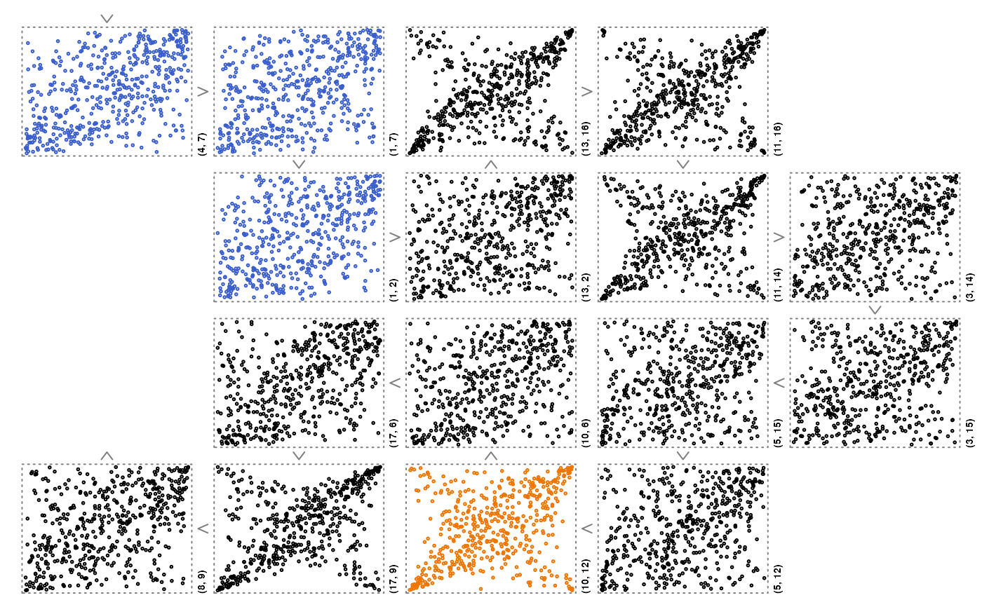
 my_points_2d_grid <- function(zargs, basecol, d.) {
r <- extract_2d(zargs)
x <- r$x; y <- r$y; xlim <- r$xlim; ylim <- r$ylim
num2d <- zargs$num/2
vars <- as.numeric(r$vlabs[num2d:(num2d+1)])
col <- if (all(1 <= vars & vars <= d.[1])) basecol[1] else
if (all(d.[1]+1 <= vars & vars <= d.[1]+d.[2])) basecol[2] else
if (all(d.[1]+d.[2]+1 <= vars & vars <= d)) basecol[3] else "black"
vp <- vport(zargs$ispace, xlim = xlim, ylim = ylim, x = x, y = y)
grid::pointsGrob(x = x[[1]], y = y[[1]],
pch = 21, size = grid::unit(0.02, "npc"),
name = "points_2d",
gp = grid::gpar(col = col), vp = vp)
}
colnames(U) <- 1:d; set.seed(1)
(ord <- sample(1:d, size = d))
#> [1] 4 7 1 2 13 16 11 14 3 15 5 12 10 6 17 9 8
zenplot(U[,ord], plot1d = "layout", plot2d = "layout", pkg = "grid")
my_points_2d_grid <- function(zargs, basecol, d.) {
r <- extract_2d(zargs)
x <- r$x; y <- r$y; xlim <- r$xlim; ylim <- r$ylim
num2d <- zargs$num/2
vars <- as.numeric(r$vlabs[num2d:(num2d+1)])
col <- if (all(1 <= vars & vars <= d.[1])) basecol[1] else
if (all(d.[1]+1 <= vars & vars <= d.[1]+d.[2])) basecol[2] else
if (all(d.[1]+d.[2]+1 <= vars & vars <= d)) basecol[3] else "black"
vp <- vport(zargs$ispace, xlim = xlim, ylim = ylim, x = x, y = y)
grid::pointsGrob(x = x[[1]], y = y[[1]],
pch = 21, size = grid::unit(0.02, "npc"),
name = "points_2d",
gp = grid::gpar(col = col), vp = vp)
}
colnames(U) <- 1:d; set.seed(1)
(ord <- sample(1:d, size = d))
#> [1] 4 7 1 2 13 16 11 14 3 15 5 12 10 6 17 9 8
zenplot(U[,ord], plot1d = "layout", plot2d = "layout", pkg = "grid")
 zenplot(U[,ord],
pkg = "grid",
plot1d = function(zargs) arrow_1d_grid(zargs, col = "grey50"),
plot2d = function(zargs)
grid::gTree(children = grid::gList(
my_points_2d_grid(zargs, basecol = basecol, d. = d.),
rect_2d_grid(zargs,
width = 1.05, height = 1.05,
col = "grey50", lty = 3),
label_2d_grid(zargs,
loc = c(1.06, -0.03),
just = c("left", "top"),
rot = 90, cex = 0.45,
fontface = "bold") )))
zenplot(U[,ord],
pkg = "grid",
plot1d = function(zargs) arrow_1d_grid(zargs, col = "grey50"),
plot2d = function(zargs)
grid::gTree(children = grid::gList(
my_points_2d_grid(zargs, basecol = basecol, d. = d.),
rect_2d_grid(zargs,
width = 1.05, height = 1.05,
col = "grey50", lty = 3),
label_2d_grid(zargs,
loc = c(1.06, -0.03),
just = c("left", "top"),
rot = 90, cex = 0.45,
fontface = "bold") )))
 # }
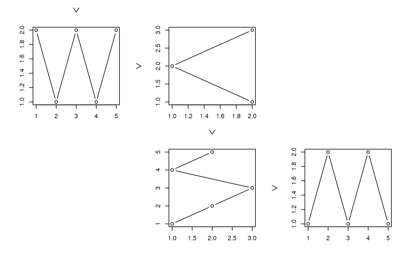
### Using ggplot2 ##############################################################
## Although not thoroughly tested, ggplot2 can be used via pkg = "grid".
# \donttest{
if (requireNamespace("ggplot2", quietly = TRUE)) {
my_points_2d_ggplot <- function(zargs, extract2d = TRUE) {
if (extract2d) {
r <- extract_2d(zargs)
df <- data.frame(r$x, r$y); names(df) <- c("x", "y")
cols <- zargs$x[,"Species"]
} else {
ii <- plot_indices(zargs)
irs <- zargs$x
df <- data.frame(x = irs[,ii[1]], y = irs[,ii[2]])
cols <- irs[,"Species"]
}
num2d <- zargs$num/2
p <- ggplot2::ggplot() +
ggplot2::geom_point(data = df,
ggplot2::aes(x = x, y = y,
colour = cols),
show.legend = (num2d == 3)) +
ggplot2::labs(x = "", y = "")
if (num2d == 3)
p <- p + ggplot2::theme(legend.position = "bottom",
legend.title = ggplot2::element_blank())
ggplot2::ggplot_gtable(ggplot2::ggplot_build(p))
}
iris. <- iris
colnames(iris.) <- gsub("\\\\.", " ", x = colnames(iris))
zenplot(iris., n2dplots = 3, plot2d = "my_points_2d_ggplot",
pkg = "grid")
zenplot(iris., n2dplots = 3,
plot2d = function(zargs) {
my_points_2d_ggplot(zargs, extract2d = FALSE)
},
pkg = "grid")
}
#> Error in zenplot(iris., n2dplots = 3, plot2d = "my_points_2d_ggplot", pkg = "grid"): Function provided as argument 'plot2d' does not exist.
# }
### Providing your own data structure ##########################################
# \donttest{
z <- list(list(1:5, 2:1, 1:3), list(1:5, 1:2))
zenplot(z, n2dplots = 4, plot1d = "arrow", last1d = FALSE,
plot2d = function(zargs, ...) {
r <- unlist(zargs$x, recursive = FALSE)
num2d <- zargs$num/2
x <- r[[num2d]]; y <- r[[num2d + 1]]
if(length(x) < length(y)) x <- rep(x, length.out = length(y))
else if(length(y) < length(x)) y <- rep(y, length.out = length(x))
plot(x, y, type = "b", xlab = "", ylab = "")
}, ispace = c(0.2, 0.2, 0.1, 0.1))
# }
### Using ggplot2 ##############################################################
## Although not thoroughly tested, ggplot2 can be used via pkg = "grid".
# \donttest{
if (requireNamespace("ggplot2", quietly = TRUE)) {
my_points_2d_ggplot <- function(zargs, extract2d = TRUE) {
if (extract2d) {
r <- extract_2d(zargs)
df <- data.frame(r$x, r$y); names(df) <- c("x", "y")
cols <- zargs$x[,"Species"]
} else {
ii <- plot_indices(zargs)
irs <- zargs$x
df <- data.frame(x = irs[,ii[1]], y = irs[,ii[2]])
cols <- irs[,"Species"]
}
num2d <- zargs$num/2
p <- ggplot2::ggplot() +
ggplot2::geom_point(data = df,
ggplot2::aes(x = x, y = y,
colour = cols),
show.legend = (num2d == 3)) +
ggplot2::labs(x = "", y = "")
if (num2d == 3)
p <- p + ggplot2::theme(legend.position = "bottom",
legend.title = ggplot2::element_blank())
ggplot2::ggplot_gtable(ggplot2::ggplot_build(p))
}
iris. <- iris
colnames(iris.) <- gsub("\\\\.", " ", x = colnames(iris))
zenplot(iris., n2dplots = 3, plot2d = "my_points_2d_ggplot",
pkg = "grid")
zenplot(iris., n2dplots = 3,
plot2d = function(zargs) {
my_points_2d_ggplot(zargs, extract2d = FALSE)
},
pkg = "grid")
}
#> Error in zenplot(iris., n2dplots = 3, plot2d = "my_points_2d_ggplot", pkg = "grid"): Function provided as argument 'plot2d' does not exist.
# }
### Providing your own data structure ##########################################
# \donttest{
z <- list(list(1:5, 2:1, 1:3), list(1:5, 1:2))
zenplot(z, n2dplots = 4, plot1d = "arrow", last1d = FALSE,
plot2d = function(zargs, ...) {
r <- unlist(zargs$x, recursive = FALSE)
num2d <- zargs$num/2
x <- r[[num2d]]; y <- r[[num2d + 1]]
if(length(x) < length(y)) x <- rep(x, length.out = length(y))
else if(length(y) < length(x)) y <- rep(y, length.out = length(x))
plot(x, y, type = "b", xlab = "", ylab = "")
}, ispace = c(0.2, 0.2, 0.1, 0.1))
 # }
### Zenplots based on 3d lattice plots #########################################
# \donttest{
if (requireNamespace("lattice", quietly = TRUE) &&
requireNamespace("gridExtra", quietly = TRUE)) {
mycloud <- function(x, num) {
lim <- extendrange(0:1, f = 0.04)
print(lattice::cloud(x[, 3] ~ x[, 1] * x[, 2],
xlim = lim, ylim = lim, zlim = lim,
xlab = substitute(U[i.], list(i. = num)),
ylab = substitute(U[i.], list(i. = num + 1)),
zlab = substitute(U[i.], list(i. = num + 2)),
zoom = 1, scales = list(arrows = FALSE, col = "black"),
col = "black",
par.settings = list(lattice::standard.theme(color = FALSE),
axis.line = list(col = "transparent"),
clip = list(panel = "off"))))
}
plst.3d <- lapply(1:4, function(i) mycloud(x[,i:(i+2)], num = i))
num <- length(plst.3d)
ncols <- 2
turns <- c(rep("r", 2*(ncols-1)), "d", "d",
rep("l", 2*(ncols-1)), "d")
plot2d <- function(zargs) {
num2d <- (zargs$num+1)/2
vp <- vport(zargs$ispace, xlim = 0:1, ylim = 0:1)
grid::grob(p = zargs$x[[num2d]], vp = vp, cl = "lattice")
}
zenplot(plst.3d, turns = turns, n2dplots = num, pkg = "grid",
first1d = FALSE, last1d = FALSE,
plot1d = "arrow_1d_grid", plot2d = plot2d)
}
# }
### Zenplots based on 3d lattice plots #########################################
# \donttest{
if (requireNamespace("lattice", quietly = TRUE) &&
requireNamespace("gridExtra", quietly = TRUE)) {
mycloud <- function(x, num) {
lim <- extendrange(0:1, f = 0.04)
print(lattice::cloud(x[, 3] ~ x[, 1] * x[, 2],
xlim = lim, ylim = lim, zlim = lim,
xlab = substitute(U[i.], list(i. = num)),
ylab = substitute(U[i.], list(i. = num + 1)),
zlab = substitute(U[i.], list(i. = num + 2)),
zoom = 1, scales = list(arrows = FALSE, col = "black"),
col = "black",
par.settings = list(lattice::standard.theme(color = FALSE),
axis.line = list(col = "transparent"),
clip = list(panel = "off"))))
}
plst.3d <- lapply(1:4, function(i) mycloud(x[,i:(i+2)], num = i))
num <- length(plst.3d)
ncols <- 2
turns <- c(rep("r", 2*(ncols-1)), "d", "d",
rep("l", 2*(ncols-1)), "d")
plot2d <- function(zargs) {
num2d <- (zargs$num+1)/2
vp <- vport(zargs$ispace, xlim = 0:1, ylim = 0:1)
grid::grob(p = zargs$x[[num2d]], vp = vp, cl = "lattice")
}
zenplot(plst.3d, turns = turns, n2dplots = num, pkg = "grid",
first1d = FALSE, last1d = FALSE,
plot1d = "arrow_1d_grid", plot2d = plot2d)
}


 # }
# }