More general smoothed density estimates

Computes and draws kernel density estimate. Compared with geom_density(), it provides more general cases that accepting x and y. See details

geom_density_(
  mapping = NULL,
  data = NULL,
  stat = "density_",
  position = "identity_",
  ...,
  scale.x = NULL,
  scale.y = c("data", "group", "variable"),
  as.mix = FALSE,
  positive = TRUE,
  prop = 0.9,
  na.rm = FALSE,
  orientation = NA,
  show.legend = NA,
  inherit.aes = TRUE
)

stat_density_(
  mapping = NULL,
  data = NULL,
  geom = "density_",
  position = "stack_",
  ...,
  bw = "nrd0",
  adjust = 1,
  kernel = "gaussian",
  n = 512,
  trim = FALSE,
  na.rm = FALSE,
  orientation = NA,
  show.legend = NA,
  inherit.aes = TRUE
)

Arguments

mapping

Set of aesthetic mappings created by aes(). If specified and inherit.aes = TRUE (the default), it is combined with the default mapping at the top level of the plot. You must supply mapping if there is no plot mapping.

data

The data to be displayed in this layer. There are three options:

If NULL, the default, the data is inherited from the plot data as specified in the call to ggplot().

A data.frame, or other object, will override the plot data. All objects will be fortified to produce a data frame. See fortify() for which variables will be created.

A function will be called with a single argument, the plot data. The return value must be a data.frame, and will be used as the layer data. A function can be created from a formula (e.g. ~ head(.x, 10)).

position

Position adjustment, either as a string naming the adjustment (e.g. "jitter" to use position_jitter), or the result of a call to a position adjustment function. Use the latter if you need to change the settings of the adjustment.

...

Other arguments passed on to layer(). These are often aesthetics, used to set an aesthetic to a fixed value, like colour = "red" or size = 3. They may also be parameters to the paired geom/stat.

scale.x

A sorted length 2 numerical vector representing the range of the whole data will be scaled to. The default value is (0, 1).

scale.y

one of data and group to specify.

Type	Description
data (default)	The density estimates are scaled by the whole data set
group	The density estimates are scaled by each group

If the scale.y is data, it is meaningful to compare the density (shape and area) across all groups; else it is only meaningful to compare the density within each group. See details.

as.mix

Logical. Within each group, if TRUE, the sum of the density estimate area is mixed and scaled to maximum 1. The area of each subgroup (in general, within each group one color represents one subgroup) is proportional to the count; if FALSE the area of each subgroup is the same, with maximum 1. See details.

positive

If y is set as the density estimate, where the smoothed curved is faced to, right (`positive`) or left (`negative`) as vertical layout; up (`positive`) or down (`negative`) as horizontal layout?

prop

adjust the proportional maximum height of the estimate (density, histogram, ...).

na.rm

If FALSE, the default, missing values are removed with a warning. If TRUE, missing values are silently removed.

orientation

The orientation of the layer. The default (NA) automatically determines the orientation from the aesthetic mapping. In the rare event that this fails it can be given explicitly by setting orientation to either "x" or "y". See the Orientation section for more detail.

show.legend

logical. Should this layer be included in the legends? NA, the default, includes if any aesthetics are mapped. FALSE never includes, and TRUE always includes. It can also be a named logical vector to finely select the aesthetics to display.

inherit.aes

If FALSE, overrides the default aesthetics, rather than combining with them. This is most useful for helper functions that define both data and aesthetics and shouldn't inherit behaviour from the default plot specification, e.g. borders().

geom, stat

Use to override the default connection between geom_density() and stat_density().

bw

The smoothing bandwidth to be used. If numeric, the standard deviation of the smoothing kernel. If character, a rule to choose the bandwidth, as listed in stats::bw.nrd().

adjust

A multiplicate bandwidth adjustment. This makes it possible to adjust the bandwidth while still using the a bandwidth estimator. For example, adjust = 1/2 means use half of the default bandwidth.

kernel

Kernel. See list of available kernels in density().

n

number of equally spaced points at which the density is to be estimated, should be a power of two, see density() for details

trim

If FALSE, the default, each density is computed on the full range of the data. If TRUE, each density is computed over the range of that group: this typically means the estimated x values will not line-up, and hence you won't be able to stack density values. This parameter only matters if you are displaying multiple densities in one plot or if you are manually adjusting the scale limits.

Details

The x (or y) is a group variable (categorical) and y (or x) is the target variable (numerical) to be plotted. If only one of x or y is provided, it will treated as a target variable and ggplot2::geom_density will be executed.

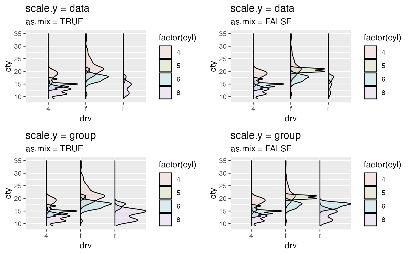
There are four combinations of scale.y and as.mix.

scale.y = "group" and as.mix = FALSE: The density estimate area of each subgroup (represented by each color) within the same group is the same.
scale.y = "group" and as.mix = TRUE: The density estimate area of each subgroup (represented by each color) within the same group is proportional to its own counts.
scale.y = "data" and as.mix = FALSE: The sum of density estimate area of all groups is scaled to maximum of 1. and the density area for each group is proportional to the its count. Within each group, the area of each subgroup is the same.
scale.y = "data" and as.mix = TRUE: The sum of density estimate area of all groups is scaled to maximum of 1 and the area of each subgroup (represented by each color) is proportional to its own count.

See vignettes[https://great-northern-diver.github.io/ggmulti/articles/histogram-density-.html] for more intuitive explanation.

Orientation

This geom treats each axis differently and, thus, can thus have two orientations. Often the orientation is easy to deduce from a combination of the given mappings and the types of positional scales in use. Thus, ggplot2 will by default try to guess which orientation the layer should have. Under rare circumstances, the orientation is ambiguous and guessing may fail. In that case the orientation can be specified directly using the orientation parameter, which can be either "x" or "y". The value gives the axis that the geom should run along, "x" being the default orientation you would expect for the geom.

Examples

if(require(dplyr)) {
  mpg %>%
    dplyr::filter(drv != "f") %>%
    ggplot(mapping = aes(x = drv, y = cty, fill = factor(cyl))) +
    geom_density_(alpha = 0.1)

  # only `x` or `y` is provided
  # that would be equivalent to call function `geom_density()`
  diamonds %>%
    dplyr::sample_n(500) %>%
    ggplot(mapping = aes(x = price)) +
    geom_density_()

  # density and boxplot
  # set the density estimate on the left
  mpg %>%
    dplyr::filter(drv != "f") %>%
    ggplot(mapping = aes(x = drv, y = cty,
                         fill = factor(cyl))) +
    geom_density_(alpha = 0.1,
                  scale.y = "group",
                  as.mix = FALSE,
                  positive = FALSE) +
    geom_boxplot()

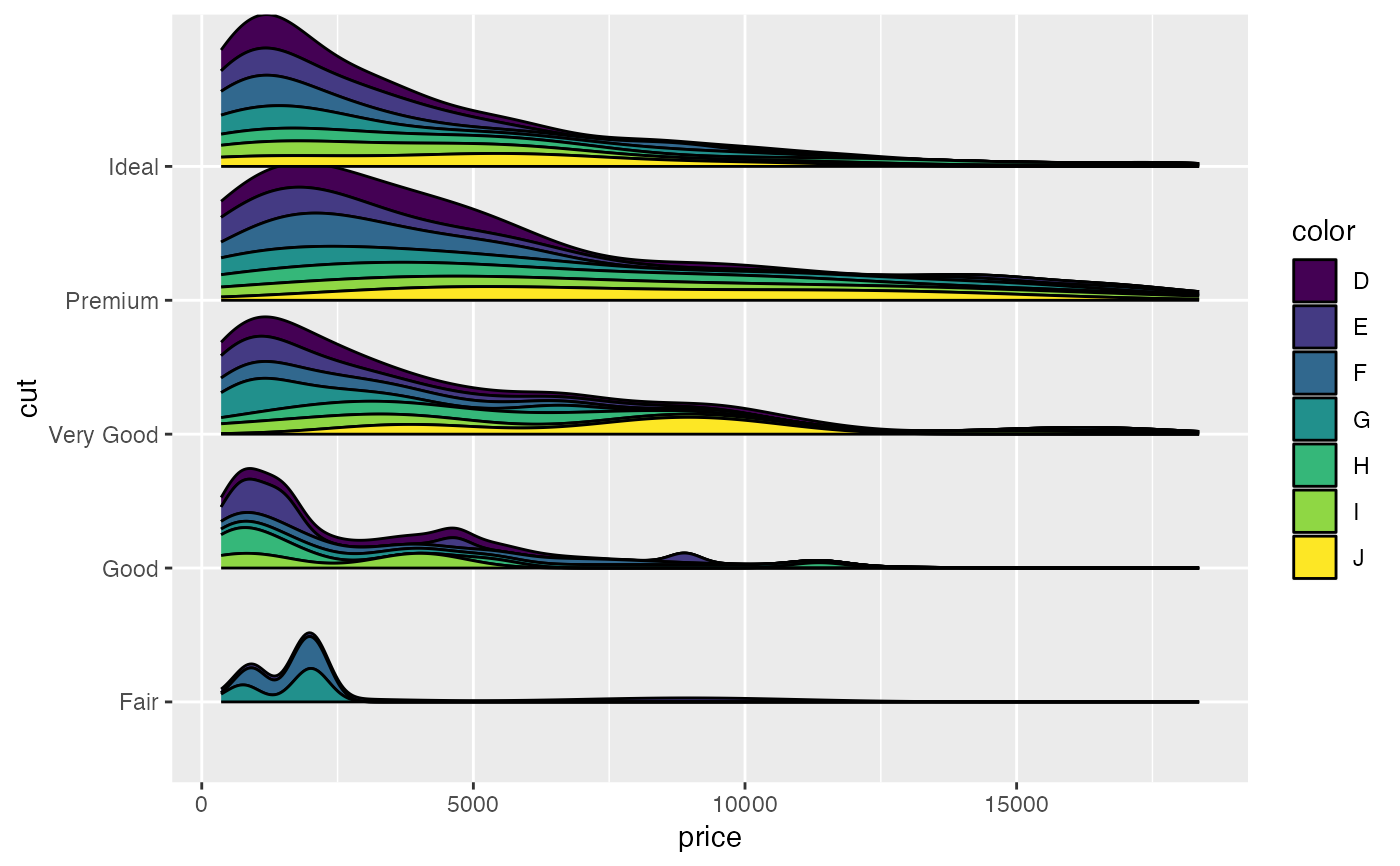
  # x as density
  set.seed(12345)
  suppressWarnings(
    diamonds %>%
      dplyr::sample_n(500) %>%
      ggplot(mapping = aes(x = price, y = cut, fill = color)) +
      geom_density_(orientation = "x", prop = 0.25,
                    position = "stack_",
                    scale.y = "group")
  )
}
#> Warning: Groups with fewer than two data points have been dropped.
#> Warning: Groups with fewer than two data points have been dropped.
#> Warning: Removed 2 rows containing missing values (`position_stack()`).

# settings of `scale.y` and `as.mix`
# \donttest{
ggplots <- lapply(list(
                      list(scale.y = "data", as.mix = TRUE),
                      list(scale.y = "data", as.mix = FALSE),
                      list(scale.y = "group", as.mix = TRUE),
                      list(scale.y = "group", as.mix = FALSE)
                    ),
                   function(vars) {
                     scale.y <- vars[["scale.y"]]
                     as.mix <- vars[["as.mix"]]
                     ggplot(mpg,
                            mapping = aes(x = drv, y = cty, fill = factor(cyl))) +
                       geom_density_(alpha = 0.1, scale.y = scale.y, as.mix = as.mix) +
                       labs(title = paste("scale.y =", scale.y),
                            subtitle = paste("as.mix =", as.mix))
                   })
suppressWarnings(
  gridExtra::grid.arrange(grobs = ggplots)
)# }

Arguments

Details

Orientation

See also

Examples