More general histogram

More general histogram (geom_histogram) or bar plot (geom_bar). Both x and y could be accommodated. See details

geom_hist_(
  mapping = NULL,
  data = NULL,
  stat = "hist_",
  position = "stack_",
  ...,
  scale.x = NULL,
  scale.y = c("data", "group", "variable"),
  as.mix = FALSE,
  binwidth = NULL,
  bins = NULL,
  positive = TRUE,
  prop = 0.9,
  na.rm = FALSE,
  orientation = NA,
  show.legend = NA,
  inherit.aes = TRUE
)

geom_histogram_(
  mapping = NULL,
  data = NULL,
  stat = "bin_",
  position = "stack_",
  ...,
  scale.x = NULL,
  scale.y = c("data", "group"),
  as.mix = FALSE,
  positive = TRUE,
  prop = 0.9,
  binwidth = NULL,
  bins = NULL,
  na.rm = FALSE,
  orientation = NA,
  show.legend = NA,
  inherit.aes = TRUE
)

geom_bar_(
  mapping = NULL,
  data = NULL,
  stat = "count_",
  position = "stack_",
  ...,
  scale.x = NULL,
  scale.y = c("data", "group"),
  positive = TRUE,
  prop = 0.9,
  na.rm = FALSE,
  orientation = NA,
  show.legend = NA,
  inherit.aes = TRUE
)

stat_hist_(
  mapping = NULL,
  data = NULL,
  geom = "bar_",
  position = "stack_",
  ...,
  binwidth = NULL,
  bins = NULL,
  center = NULL,
  boundary = NULL,
  breaks = NULL,
  closed = c("right", "left"),
  pad = FALSE,
  width = NULL,
  na.rm = FALSE,
  orientation = NA,
  show.legend = NA,
  inherit.aes = TRUE
)

stat_bin_(
  mapping = NULL,
  data = NULL,
  geom = "bar_",
  position = "stack_",
  ...,
  binwidth = NULL,
  bins = NULL,
  center = NULL,
  boundary = NULL,
  breaks = NULL,
  closed = c("right", "left"),
  pad = FALSE,
  na.rm = FALSE,
  orientation = NA,
  show.legend = NA,
  inherit.aes = TRUE
)

stat_count_(
  mapping = NULL,
  data = NULL,
  geom = "bar_",
  position = "stack_",
  ...,
  width = NULL,
  na.rm = FALSE,
  orientation = NA,
  show.legend = NA,
  inherit.aes = TRUE
)

Arguments

mapping

Set of aesthetic mappings created by aes(). If specified and inherit.aes = TRUE (the default), it is combined with the default mapping at the top level of the plot. You must supply mapping if there is no plot mapping.

data

The data to be displayed in this layer. There are three options:

If NULL, the default, the data is inherited from the plot data as specified in the call to ggplot().

A data.frame, or other object, will override the plot data. All objects will be fortified to produce a data frame. See fortify() for which variables will be created.

A function will be called with a single argument, the plot data. The return value must be a data.frame, and will be used as the layer data. A function can be created from a formula (e.g. ~ head(.x, 10)).

position

Position adjustment, either as a string, or the result of a call to a position adjustment function. Function geom_hist_ and geom_histogram_ understand stack_ (stacks bars on top of each other), or dodge_ and dodge2_ (overlapping objects side-to-side) instead of stack, dodge or dodge2

...

Other arguments passed on to layer(). These are often aesthetics, used to set an aesthetic to a fixed value, like colour = "red" or size = 3. They may also be parameters to the paired geom/stat.

scale.x

A sorted length 2 numerical vector representing the range of the whole data will be scaled to. The default value is (0, 1).

scale.y

one of data and group to specify.

Type	Description
data (default)	The density estimates are scaled by the whole data set
group	The density estimates are scaled by each group

If the scale.y is data, it is meaningful to compare the density (shape and area) across all groups; else it is only meaningful to compare the density within each group. See details.

as.mix

Logical. Within each group, if TRUE, the sum of the density estimate area is mixed and scaled to maximum 1. The area of each subgroup (in general, within each group one color represents one subgroup) is proportional to the count; if FALSE the area of each subgroup is the same, with maximum 1. See details.

binwidth

The width of the bins. Can be specified as a numeric value or as a function that calculates width from unscaled x. Here, "unscaled x" refers to the original x values in the data, before application of any scale transformation. When specifying a function along with a grouping structure, the function will be called once per group. The default is to use the number of bins in bins, covering the range of the data. You should always override this value, exploring multiple widths to find the best to illustrate the stories in your data.

The bin width of a date variable is the number of days in each time; the bin width of a time variable is the number of seconds.

bins

Number of bins. Overridden by binwidth. Defaults to 30.

positive

If y is set as the density estimate, where the smoothed curved is faced to, right (`positive`) or left (`negative`) as vertical layout; up (`positive`) or down (`negative`) as horizontal layout?

prop

adjust the proportional maximum height of the estimate (density, histogram, ...).

na.rm

If FALSE, the default, missing values are removed with a warning. If TRUE, missing values are silently removed.

orientation

The orientation of the layer. The default (NA) automatically determines the orientation from the aesthetic mapping. In the rare event that this fails it can be given explicitly by setting orientation to either "x" or "y". See the Orientation section for more detail.

show.legend

logical. Should this layer be included in the legends? NA, the default, includes if any aesthetics are mapped. FALSE never includes, and TRUE always includes. It can also be a named logical vector to finely select the aesthetics to display.

inherit.aes

If FALSE, overrides the default aesthetics, rather than combining with them. This is most useful for helper functions that define both data and aesthetics and shouldn't inherit behaviour from the default plot specification, e.g. borders().

geom, stat

Use to override the default connection between geom_hist_()/geom_histogram_()/geom_bar_() and stat_hist_()/stat_bin_()/stat_count_().

center, boundary

bin position specifiers. Only one, center or boundary, may be specified for a single plot. center specifies the center of one of the bins. boundary specifies the boundary between two bins. Note that if either is above or below the range of the data, things will be shifted by the appropriate integer multiple of binwidth. For example, to center on integers use binwidth = 1 and center = 0, even if 0 is outside the range of the data. Alternatively, this same alignment can be specified with binwidth = 1 and boundary = 0.5, even if 0.5 is outside the range of the data.

breaks

Alternatively, you can supply a numeric vector giving the bin boundaries. Overrides binwidth, bins, center, and boundary.

closed

One of "right" or "left" indicating whether right or left edges of bins are included in the bin.

pad

If TRUE, adds empty bins at either end of x. This ensures frequency polygons touch 0. Defaults to FALSE.

width

Bar width. By default, set to 90% of the resolution() of the data.

Details

x (or y) is a group variable (categorical) and y (or x) a target variable (numerical) to be plotted. If only one of x or y is provided, it will treated as a target variable and ggplot2::geom_histogram will be executed. Several things should be noticed:

1. If both x and y are given, they can be one discrete one continuous or two discrete. But they cannot be two continuous variables (which one will be considered as a group variable?).

2. geom_hist_ is a wrapper of geom_histogram_ and geom_count_. Suppose the y is our interest (x is the categorical variable), geom_hist_() can accommodate either continuous or discrete y. While, geom_histogram_() only accommodates the continuous y and geom_bar_() only accommodates the discrete y.

3. There are four combinations of scale.y and as.mix.

scale.y = "group" and as.mix = FALSE: The density estimate area of each subgroup (represented by each color) within the same group is the same.
scale.y = "group" and as.mix = TRUE: The density estimate area of each subgroup (represented by each color) within the same group is proportional to its own counts.
scale.y = "data" and as.mix = FALSE: The sum of density estimate area of all groups is scaled to maximum of 1. and the density area for each group is proportional to the its count. Within each group, the area of each subgroup is the same.
scale.y = "data" and as.mix = TRUE: The sum of density estimate area of all groups is scaled to maximum of 1 and the area of each subgroup (represented by each color) is proportional to its own count.

See vignettes[https://great-northern-diver.github.io/ggmulti/articles/histogram-density-.html] for more intuitive explanation. Note that, if it is a grouped bar chart (both x and y are categorical), parameter `as.mix` is meaningless.

Orientation

This geom treats each axis differently and, thus, can thus have two orientations. Often the orientation is easy to deduce from a combination of the given mappings and the types of positional scales in use. Thus, ggplot2 will by default try to guess which orientation the layer should have. Under rare circumstances, the orientation is ambiguous and guessing may fail. In that case the orientation can be specified directly using the orientation parameter, which can be either "x" or "y". The value gives the axis that the geom should run along, "x" being the default orientation you would expect for the geom.

Examples

if(require(dplyr) && require(tidyr)) {

  # histogram
  p0 <- mpg %>%
    dplyr::filter(manufacturer %in% c("dodge", "ford", "toyota", "volkswagen")) %>%
    ggplot(mapping = aes(x = manufacturer, y = cty))
  p0 + geom_hist_()

  ## set position
  #### default is "stack_"
  p0 + geom_hist_(mapping = aes(fill = fl))
  #### "dodge_"
  p0 + geom_hist_(position = "dodge_",
                  mapping = aes(fill = fl))
  #### "dodge2_"
  p0 + geom_hist_(position = "dodge2_",
                  mapping = aes(fill = fl))

  # bar chart
  mpg %>%
    ggplot(mapping = aes(x = drv, y = class)) +
    geom_hist_(orientation = "y")

  # scale.y as "group"
  p <- iris %>%
    tidyr::pivot_longer(cols = -Species,
                        names_to = "Outer sterile whorls",
                        values_to = "x") %>%
    ggplot(mapping = aes(x = `Outer sterile whorls`,
                         y = x, fill = Species)) +
    stat_hist_(scale.y = "group",
               prop = 0.6,
               alpha = 0.5)
  p
  # with density on the left
  p + stat_density_(scale.y = "group",
                    prop = 0.6,
                    alpha = 0.5,
                    positive = FALSE)

  ########### only `x` or `y` is provided ###########
  # that would be equivalent to call function
  # `geom_histogram()` or `geom_bar()`
  ### histogram
  diamonds %>%
    dplyr::sample_n(500) %>%
    ggplot(mapping = aes(x = price)) +
    geom_hist_()
  ### bar chart
  diamonds %>%
    dplyr::sample_n(500) %>%
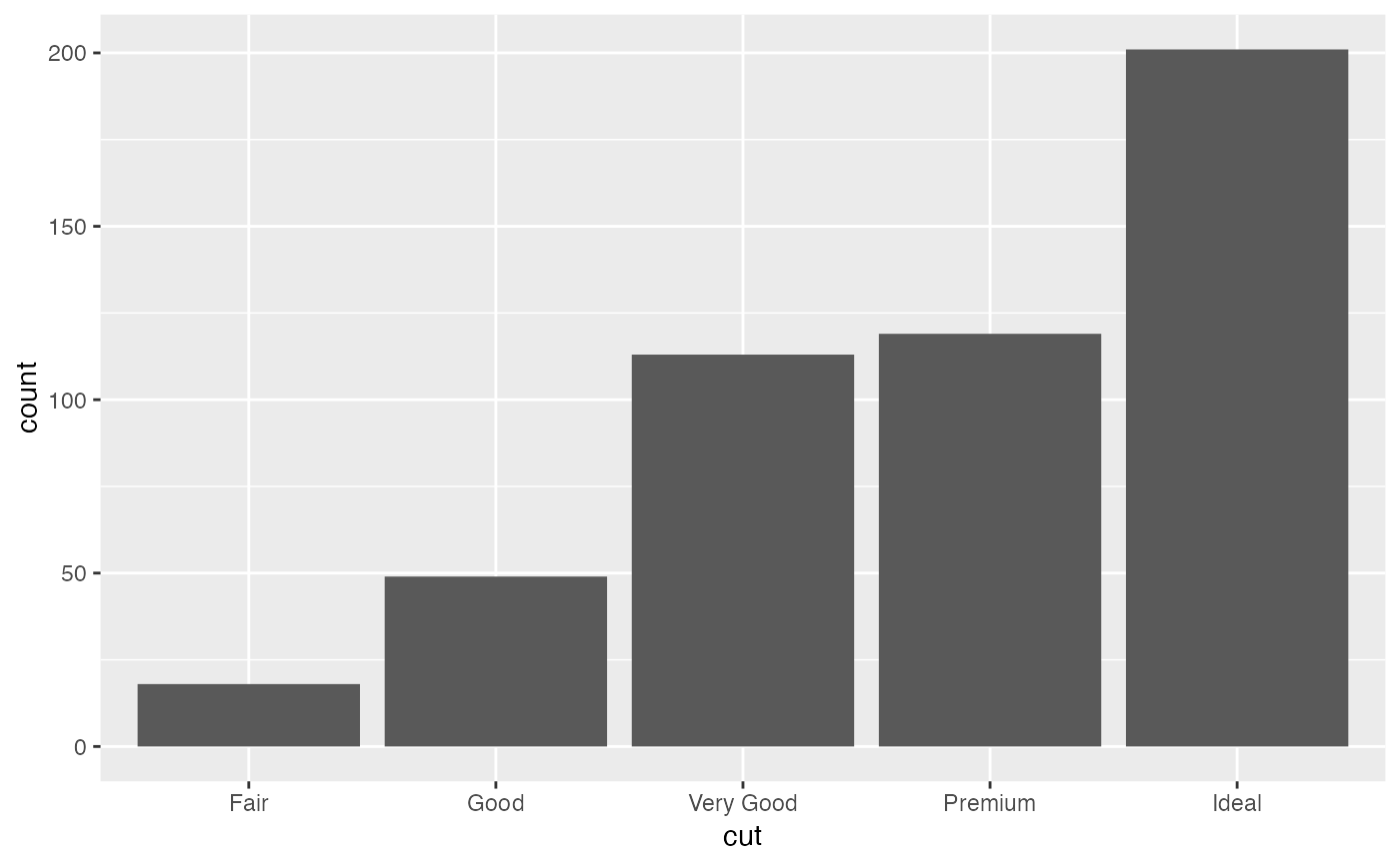
    ggplot(mapping = aes(x = cut)) +
    geom_hist_()
}
#> Loading required package: tidyr

Arguments

Details

Orientation

See also

Examples