Create an interactive loon plot widget

l_plot is a generic function for creating an interactive visualization environments for R objects.

l_plot(x, y, ...)

# S3 method for default
l_plot(
  x,
  y = NULL,
  by = NULL,
  on,
  layout = c("grid", "wrap", "separate"),
  connectedScales = c("cross", "row", "column", "both", "x", "y", "none"),
  color = l_getOption("color"),
  glyph = l_getOption("glyph"),
  size = l_getOption("size"),
  active = TRUE,
  selected = FALSE,
  xlabel,
  ylabel,
  title,
  showLabels = TRUE,
  showScales = FALSE,
  showGuides = TRUE,
  guidelines = l_getOption("guidelines"),
  guidesBackground = l_getOption("guidesBackground"),
  foreground = l_getOption("foreground"),
  background = l_getOption("background"),
  parent = NULL,
  ...
)

# S3 method for decomposed.ts
l_plot(
  x,
  y = NULL,
  xlabel = NULL,
  ylabel = NULL,
  title = NULL,
  tk_title = NULL,
  color = l_getOption("color"),
  size = l_getOption("size"),
  linecolor = l_getOption("color"),
  linewidth = l_getOption("linewidth"),
  linkingGroup,
  showScales = TRUE,
  showGuides = TRUE,
  showLabels = TRUE,
  ...
)

# S3 method for density
l_plot(
  x,
  y = NULL,
  xlabel = NULL,
  ylabel = NULL,
  title = NULL,
  linewidth = l_getOption("linewidth"),
  linecolor = l_getOption("color"),
  ...
)

# S3 method for map
l_plot(x, y = NULL, ...)

# S3 method for stl
l_plot(
  x,
  y = NULL,
  xlabel = NULL,
  ylabel = NULL,
  title = NULL,
  tk_title = NULL,
  color = l_getOption("color"),
  size = l_getOption("size"),
  linecolor = l_getOption("color"),
  linewidth = l_getOption("linewidth"),
  linkingGroup,
  showScales = TRUE,
  showGuides = TRUE,
  showLabels = TRUE,
  ...
)

Arguments

x	the coordinates of points in the l_plot. Alternatively, a single plotting structure (see the function xy.coords for details), formula, or any R object (e.g. density,stl, etc) is accommodated.
y	the y coordinates of points in the l_plot, optional if x is an appropriate structure.
...	named arguments to modify plot states. See l_info_states of any instantiated l_plot for examples of names and values.
by	loon plot can be separated by some variables into multiple panels. This argument can take a formula, n dimensional state names (see l_nDimStateNames) an n-dimensional vector and data.frame or a list of same lengths n as input.
on	if the x or by is a formula, an optional data frame containing the variables in the x or by. If the variables are not found in data, they are taken from environment, typically the environment from which the function is called.
layout	layout facets as 'grid', 'wrap' or 'separate'
connectedScales	Determines how the scales of the facets are to be connected depending on which layout is used. For each value of layout, the scales are connected as follows: layout = "wrap": Across all facets, when connectedScales is "x", then only the "x" scales are connected "y", then only the "y" scales are connected "both", both "x" and "y" scales are connected "none", neither "x" nor "y" scales are connected. For any other value, only the "y" scale is connected. layout = "grid": Across all facets, when connectedScales is "cross", then only the scales in the same row and the same column are connected "row", then both "x" and "y" scales of facets in the same row are connected "column", then both "x" and "y" scales of facets in the same column are connected "x", then all of the "x" scales are connected (regardless of column) "y", then all of the "y" scales are connected (regardless of row) "both", both "x" and "y" scales are connected in all facets "none", neither "x" nor "y" scales are connected in any facets.
color	colours of points; colours are repeated until matching the number points. Default is found using l_getOption("color").
glyph	the visual representation of the point. Argument values can be any of the string names of primitive glyphs: circles: "circle", "ccircle", "ocircle"; squares or boxes: "square", "csquare", "osquare"; triangles: "triangle", "ctriangle", "otriangle"; diamonds: "diamond", "cdiamond", or "odiamond". Note that prefixes "c" and "o" may be thought of as closed and open, respectively. The set of values are returned by l_primitiveGlyphs(). the string names of constructed glyphs: text as glyphs: see l_glyph_add_text() point ranges: see l_glyph_add_pointrange() polygons: see l_glyph_add_polygon() parallel coordinates: see l_glyph_add_serialaxes() star or radial axes: see l_glyph_add_serialaxes() or any plot created using R: see l_make_glyphs() Note that glyphs are constructed and given a stringname to be used in the inspector.
size	size of the symbol (roughly in terms of area). Default is found using l_getOption("size").
active	a logical determining whether points appear or not (default is TRUE for all points). If a logical vector is given of length equal to the number of points, then it identifies which points appear (TRUE) and which do not (FALSE).
selected	a logical determining whether points appear selected at first (default is FALSE for all points). If a logical vector is given of length equal to the number of points, then it identifies which points are (TRUE) and which are not (FALSE).
xlabel	Label for the horizontal (x) axis. If missing, one will be inferred from x if possible.
ylabel	Label for the vertical (y) axis. If missing, one will be inferred from y (or x) if possible.
title	Title for the plot, default is an empty string.
showLabels	logical to determine whether axes label (and title) should be presented.
showScales	logical to determine whether numerical scales should be presented on both axes.
showGuides	logical to determine whether to present background guidelines to help determine locations.
guidelines	colour of the guidelines shown when showGuides = TRUE. Default is found using l_getOption("guidelines").
guidesBackground	colour of the background to the guidelines shown when showGuides = TRUE. Default is found using l_getOption("guidesBackground").
foreground	foreground colour used by all other drawing. Default is found using l_getOption("foreground").
background	background colour used for the plot. Default is found using l_getOption("background").
parent	a valid Tk parent widget path. When the parent widget is specified (i.e. not NULL) then the plot widget needs to be placed using some geometry manager like tkpack or tkplace in order to be displayed. See the examples below.
tk_title	provides an alternative window name to Tk's wm title. If NULL, stl will be used.
linecolor	line colour of all time series. Default given by l_getOption("color").
linewidth	line width of all time series (incl. original and decomposed components. Default given by l_getOption("linewidth").
linkingGroup	string giving the linkingGroup for all plots. If missing, a default linkingGroup will be determined from deparsing the input x.

Value

• The input is a stl or a decomposed.ts object, a structure of class "l_ts" containing four loon plots each representing a part of the decomposition by name: "original", "trend", "seasonal", and "remainder"

• The input is a vector, formula, data.frame, ...

  • by = NULL: a loon widget will be returned

  • by is not NULL: an l_facet object (a list) will be returned and each element is a loon widget displaying a subset of interest.

Details

Like plot in R, l_plot is the generic plotting function for objects in loon. The default method l_plot.default produces the interactive scatterplot in loon. This is the workhorse of `loon` and is often a key part of many other displays (e.g. l_pairs and l_navgraph).

For example, the methods include l_plot.default (the basic interactive scatterplot), l_plot.density (layers output of density in an empty scatterplot), l_plot.map (layers a map in an empty scatterplot), and l_plot.stl (a compound display of the output of stl).

A complete list is had from methods(l_plot).

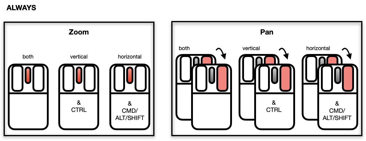
To get started with loon it is recommended to follow the introductory loon vignette vignette(topic = "introduction", package = "loon") and to explore loon's website accessible via l_help().

The general direct manipulation and interaction gestures are outlined in the following figures.

Zooming and Panning

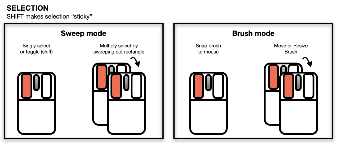
Selecting Points/Objects

Moving Points on the Scatterplot Display

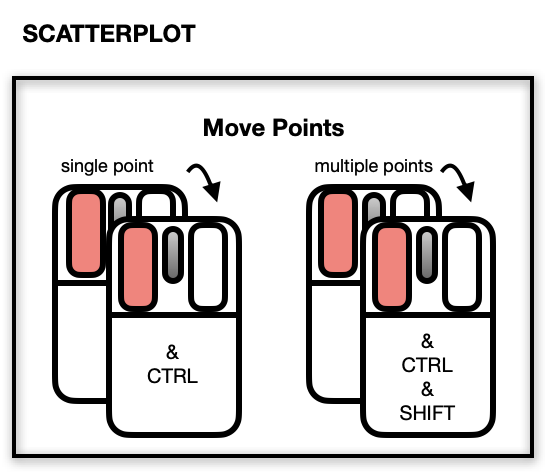
The scatterplot displays a number of direct interactions with the mouse and keyboard, these include: zooming towards the mouse cursor using the mouse wheel, panning by right-click dragging and various selection methods using the left mouse button such as sweeping, brushing and individual point selection. See the documentation for l_plot for more details about the interaction gestures.

Some arguments to modify layouts can be passed through, e.g. "separate", "ncol", "nrow", etc. Check l_facet to see how these arguments work.

See also

Turn interactive loon plot static loonGrob, grid.loon, plot.loon.

Density layer l_layer.density

Map layer l_layer, l_layer.map, map

Other loon interactive states: l_hist(), l_info_states(), l_serialaxes(), l_state_names(), names.loon()

Examples

if(interactive()) {
########################## l_plot.default ##########################
# default use as scatterplot

p1 <- with(iris, l_plot(Sepal.Length, Sepal.Width, color=Species,
                        title = "First plot"))

# The names of the info states that can be
# accessed or set.  They can also be given values as
# arguments to l_plot.default()
names(p1)
p1["size"] <- 10

p2 <- with(iris, l_plot(Petal.Length ~ Petal.Width,
                        linkingGroup="iris_data",
                        title = "Second plot",
                        showGuides = FALSE))
p2["showScales"] <- TRUE

# link first plot with the second plot requires
# l_configure to coordinate the synchroniztion
l_configure(p1, linkingGroup = "iris_data", sync = "push")

p1['selected'] <- iris$Species == "versicolor"
p2["glyph"][p1['selected']] <- "cdiamond"

gridExtra::grid.arrange(loonGrob(p1), loonGrob(p2), nrow = 1)

# Layout facets
### facet wrap
p3 <- with(mtcars, l_plot(wt, mpg, by = cyl, layout = "wrap"))
# it is equivalent to
# p3 <- l_plot(mpg~wt, by = ~cyl, layout = "wrap", on = mtcars)

### facet grid
p4 <- l_plot(x = 1:6, y = 1:6,
             by = size ~ color,
             size = c(rep(50, 2), rep(25, 2), rep(50, 2)),
             color = c(rep("red", 3), rep("green", 3)))

# Use with other tk widgets
tt <- tktoplevel()
tktitle(tt) <- "Loon plots with custom layout"

p1 <- l_plot(parent=tt, x=c(1,2,3), y=c(3,2,1))
p2 <- l_plot(parent=tt, x=c(4,3,1), y=c(6,8,4))

tkgrid(p1, row=0, column=0, sticky="nesw")
tkgrid(p2, row=0, column=1, sticky="nesw")

tkgrid.columnconfigure(tt, 0, weight=1)
tkgrid.columnconfigure(tt, 1, weight=1)

tkgrid.rowconfigure(tt, 0, weight=1)
########################## l_plot.decomposed.ts ##########################
decompose <- decompose(co2)
p <- l_plot(decompose, title = "Atmospheric carbon dioxide over Mauna Loa")
# names of plots in the display
names(p)
# names of states associated with the seasonality plot
names(p$seasonal)
# which can be set
p$seasonal['color'] <- "steelblue"

########################## l_plot.stl ##########################
co2_stl <- stl(co2, "per")
p <- l_plot(co2_stl, title = "Atmospheric carbon dioxide over Mauna Loa")
# names of plots in the display
names(p)
# names of states associated with the seasonality plot
names(p$seasonal)
# which can be set
p$seasonal['color'] <- "steelblue"
########################## l_plot.density ##########################
# plot a density estimate
set.seed(314159)
ds <- density(rnorm(1000))
p <- l_plot(ds,  title = "density estimate",
            xlabel = "x", ylabel = "density",
            showScales = TRUE)

########################## l_plot.map ##########################
if (requireNamespace("maps", quietly = TRUE)) {
   p <- l_plot(maps::map('world', fill=TRUE, plot=FALSE))
}
}