library(loon.tourr)Introduction
A tour is a motion graphic designed to study the joint distribution of multivariate data (Asimov 1985)(Andreas Buja and Asimov 1986). A sequence of low-dimensional projections is created by a high dimensional data set. Tours are thus used to find interesting projections. Between each plane, interpolation along a geodesic path is provided so that the points in a sub space (e.g. 2D) can be rotated smoothly. In mathematics, \(\boldsymbol{X}_{n \times p}\) represents the original data set; \(\boldsymbol{P}_{p \times d}\) is the matrix of projection vectors where \(d < p\). [ = ] where \(\boldsymbol{Y}\) is the lower dimensional sub-space.
The tour was first implemented in the software Dataviewer (A. Buja, Asimov, and Hurley 1986)(Hurley 1987)(Andreas Buja, Hurley, and McDonald 1987) in Symbolics Lisp machine. A smoothly moving scatterplot could be produced to visualize the tour paths. Then, D. F. Swayne, Cook, and Buja (1991) implemented software XGobi in the X Window System, providing portability across a wide variety of workstations i.e. X terminals, personal computers, even across a network. Software GGobi (D. Swayne et al. 2001)(Cook, Swayne, and Buja 2007), redesigned and extended its ancestor XGobi. It can be embedded in other software, like environment R. Package rggobi (Lang et al. 2018) is an R interface of GGobi, however, it has been removed from the CRAN and can only be accessed from the archive.
Package tourr (Wickham et al. 2011) implements geodesic interpolation and variety tour generation functions (i.e. grand tour, guided tour, etc) in R language. The function animate provides tour animation as a kinematic sequence of static displays – plots are generated and then displayed quickly in order. In an RStudio display, for example, the user can cycle back and forth through the sequence … but that is all. Unlike earlier tour implementations (rggobi) no interactive manipulation of the plot elements is possible.
The loon package (Waddell and Oldford 2020) is a toolkit that enables highly interactive data visualization. The package loon.tourr adds the full functionality of loon’s interactive graphics to tourr. For example, this allows interactive selection, colouring, and deactivating of points in the tour display and linking that display with any other loon plot. Interesting projections discovered during the tour can be accessed at any point in the tour. In addition, random tours displaying more than 2 dimensions are also provided using parallel or radial coordinates and scatterplot matrices.
Basics
The crabs (Campbell and Mahon 1974) data frame (stored in package MASS) contains 200 observations and 8 features, describing 5 morphological measurements on 50 crabs each of two colour forms and both sexes. GIF 1 shows the tours and color represents the species, “B” (blue) or “O” (orange).
| sp | sex | index | FL | RW | CL | CW | BD |
|---|---|---|---|---|---|---|---|
| B | M | 1 | 8.1 | 6.7 | 16.1 | 19.0 | 7.0 |
| B | M | 2 | 8.8 | 7.7 | 18.1 | 20.8 | 7.4 |
| B | M | 3 | 9.2 | 7.8 | 19.0 | 22.4 | 7.7 |
| B | M | 4 | 9.6 | 7.9 | 20.1 | 23.1 | 8.2 |
| B | M | 5 | 9.8 | 8.0 | 20.3 | 23.0 | 8.2 |
| B | M | 6 | 10.8 | 9.0 | 23.0 | 26.5 | 9.8 |
This plot is interactive. Users can pan, zoom or select on this plot. The default number of random bases is 30 and the steps between two serial projections are 40. So, we have 1200 + 1 (start position) projections in total. To navigate the tour, scroll the rightmost bar down, the projection is transformed from one to another. If, unfortunately, none of the projections is interesting, click the “refresh” button at the left-bottom corner. New random tours are created.
Immediately below the plot, behind the “refresh” button, there are several radio buttons, “data,” “variable,” “observation” and “sphere” that represent the scaling methods \(f\) of \(\boldsymbol{X}\).
The first of which is “data,” where \(f(\boldsymbol{X}) = \boldsymbol{X}\);
If
scaling = "variable", \(f(\mathbf{x}_j) = \frac{1}{a - b}(\mathbf{x}_j - b\mathbf{1})\) where \(\boldsymbol{X} = [\mathbf{x}_{1}, ..., \mathbf{x}_{p}]\), \(\mathbf{x}_{j}\) is a \(n \times 1\) vector, \(a = \max{(\mathbf{x}_j)}\) and \(b = \min{(\mathbf{x}_j)}\);The third is “observation,” where \(f(\mathbf{x}_i) = \frac{1}{c - d}(\mathbf{x}_i - d\mathbf{1})\), \(\boldsymbol{X} = {[{\mathbf{x}_{1}}^{\mkern-1.5mu\mathsf{T}}, ..., {\mathbf{x}_{n}}^{\mkern-1.5mu\mathsf{T}}]}^{\mkern-1.5mu\mathsf{T}}\), \(\mathbf{x}_{i}\) is a \(p \times 1\) vector, \(c = \max{(\mathbf{x}_i)}\) and \(d = \min{(\mathbf{x}_i)}\);
If the scaling method is “sphere,” where \(f(\boldsymbol{X}) = \boldsymbol{X}^\star \boldsymbol{V}\) where \(\boldsymbol{X}^\star = (\boldsymbol{I} - \frac{1}{n}\mathbf{1}{\mathbf{1}}^{\mkern-1.5mu\mathsf{T}})\boldsymbol{X} = \boldsymbol{U} \boldsymbol{D} \boldsymbol{V}\).
Notice that the tour is based on the transformed data set [ = f() ]
color <- rep("skyblue", nrow(crabs))
color[crabs$sp == "O"] <- "orange"
cr <- crabs[, c("FL", "RW", "CL", "CW", "BD")]
p0 <- l_tour(cr, color = color)
GIF 1: 2D grand tour
The projection dimension (the dimension of the \(\boldsymbol{P}\)) is controlled by tour_path = grand_tour(d) where \(d\) represents the dimensions and the default is \(2\). Unlike the 2 dimensional Cartesian coordinate, higher dimensional space (\(>2\)) will be embedded in the parallel coordinate or radial coordinate. In GIF 2, the \(d\) is set as 4.
p1 <- l_tour(cr,
             tour_path = grand_tour(4L),
             color = color)
GIF 2: 4D grand tour
An l_tour object is returned by p1 (or p0).
class(p1) # class(p0)
# > [1] "l_tour" "loon"
The loon serialaxes plot for p1 (or scatterplot for p0) can be accessed by calling l_getPlots
w <- l_getPlots(p1)
class(w)
# > [1] "l_serialaxes" "loon"
The matrix of projection vectors \(\boldsymbol{P}_{4 \times 4}\) can be returned by function l_cget or a simple [
round(p1["projection"], 2)
# >
#       [,1]  [,2]  [,3]  [,4]
# [1,] -0.12 -0.93 -0.01 -0.35
# [2,] -0.57  0.21  0.63 -0.36
# [3,] -0.06  0.14  0.14 -0.38
# [4,] -0.37  0.23 -0.76 -0.47
# [5,] -0.72 -0.14 -0.12  0.62
The radial coordinate can be converted to a parallel coordinate by calling [<- in the console or trigger the “parallel” radio button of “axes layout” on p1’s inspector.
p1["axesLayout"] <- "parallel"Additionally, Andrews plot can be shown by runing the following code in console
p1["andrews"] <- TRUEThe interactive graphics can be turned to static either by
plot(p1)or
loon.ggplot::loon.ggplot(p1)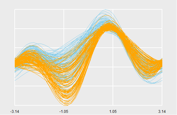
Figure 1: Andrews curve
To investigate more about loon, please visit great-northern-diver-loon.
Tour techniques
Cook, Swayne, and Buja (2007) introduced several methods for choosing projections. In loon.tourr, by modifying the argument tour_path, all can be realized.
-
Grand tour: a sequence of projections is chosen randomly
# Default, 2D grand tour pg <- l_tour(cr, tour_path = grand_tour(2L)) -
Projection pursuit guided tour: a sequence of projections is guided by an algorithm in search of “interesting” projections by optimizing a criterion function
[g(), ] where \(\boldsymbol{Y} = {[{\mathbf{y}}^{\mkern-1.5mu\mathsf{T}}_1, ..., {\mathbf{y}}^{\mkern-1.5mu\mathsf{T}}_n]}^{\mkern-1.5mu\mathsf{T}} = \boldsymbol{X} \boldsymbol{P}\), \(\mathbf{y}_j\) is a \(p \times 1\) vector.
-
Holes:
[g() = ]
# 2D holes projection pursuit indexes pp_holes <- l_tour(cr, tour_path = guided_tour(holes(), 2L)) -
Central Mass:
[g() = ]
# 2D CM projection pursuit indexes pp_CM <- l_tour(cr, tour_path = guided_tour(cmass(), 2L)) -
LDA
[g() = 1 - ]
where \(\boldsymbol{B} = \sum_{i=1}^k n_i (\bar{y}_{i.} - \bar{y}_{..}) {(\bar{y}_{i.} - \bar{y}_{..})}^{\mkern-1.5mu\mathsf{T}}\), \(\boldsymbol{W} = \sum_{i=1}^k \sum_{j=1}^{n_i} n_i (\bar{y}_{ij} - \bar{y}_{i.}) {(\bar{y}_{ij} - \bar{y}_{i.})}^{\mkern-1.5mu\mathsf{T}}\) and \(k\) is the number of groups.
# 2D LDA projection pursuit indexes
pp_LDA <- l_tour(cr,
                 color = crabs$sex,
                 tour_path = guided_tour(lda_pp(crabs$sex), 2L))
-
-
Expect these,
tourralso provides some other tour methods, for example:-
frozen_tour, one variable is designated as the “manipulation variable,” and the projection coefficient for this variable is controlled; -
little_tour, a planned tour that travels between all axis parallel projections; -
local_tour, alternates between the starting position and a nearby random projection and etc.
-
Compound plot
Facets
GIF 3 shows the tour plot separated by variable sex into two panels.
pf <- l_tour(cr,
             by = crabs$sex,
             color = color)
GIF 3: facets
Pairs plot
GIF 4 shows the tour pairs plot (the upper triangle). If we set showSerialAxes = TRUE, a serial axes plot (parallel or radial axes) is displayed at the lower triangle.
pp <- l_tour_pairs(cr,
                   tour_path = grand_tour(4L),
                   color = color,
                   showSerialAxes = TRUE)
GIF 4: pairs plot
Tour compound plot is a l_tour_compound object
class(pp) # or class(pf)
# > [1] "l_tour_compound" "loon"
The loon pairs plot can be accessed by calling l_getPlots. It will return a l_compound widget that a list contains seven loon widgets.
wp <- l_getPlots(pp)
wp
# >
# $x2y1
# [1] ".l0.pairs.plot"
# attr(,"class")
# [1] "l_plot" "loon"
#
# $x3y1
# [1] ".l0.pairs.plot1"
# attr(,"class")
# [1] "l_plot" "loon"
#
# $x4y1
# [1] ".l0.pairs.plot2"
# attr(,"class")
# [1] "l_plot" "loon"
#
# $x3y2
# [1] ".l0.pairs.plot3"
# attr(,"class")
# [1] "l_plot" "loon"
#
# $x4y2
# [1] ".l0.pairs.plot4"
# attr(,"class")
# [1] "l_plot" "loon"
#
# $x4y3
# [1] ".l0.pairs.plot5"
# attr(,"class")
# [1] "l_plot" "loon"
#
# $serialAxes
# [1] ".l0.pairs.serialaxes"
# attr(,"class")
# [1] "l_serialaxes" "loon"
#
# attr(,"class")
# [1] "l_pairs"    "l_compound" "loon"
Note that all the plots in a single compound widget share the same projection (e.g pp['projection']).
Layers
Sometimes, layering visuals in a tour is helpful to find an interesting “pattern.”
l_layer_hull
A convex hull is the smallest convex set that contains it. We can add such layer by l_layer_hull
# pack layer on top of `p0`
l0 <- l_layer_hull(p0, group = crabs$sp)
The argument group is used to clarify the group of the set in each hull. Suppose we want to find a projection that splits the crab species well, layering the hull could be extremely useful. If two hulls have no intersections, this projection could be the one we are looking for.
GIF 5: layer hull
l_layer_density2d
Two dimensional kernel density estimation can tell the dense of a distribution.
# hide the hull
l_layer_hide(l0)
# density2D
l1 <- l_layer_density2d(p0)
GIF 5: layer density
l_layer_trails
Display trails in tours
# hide the density2D
l_layer_hide(l1)
# density2D
l2 <- l_layer_trails(p0)
GIF 5: layer density
The trails can show the direction of the projection. Meanwhile, the lengths of tails represent the steps of each transformation.
Build your own layers
The interactive layers are realized by modifying function l_layer_callback. It is a generic function and the class is determined by label. For example, we want to create a static point layer and make it as a background of the object pf.
allx <- unlist(pf['x'])
ally <- unlist(pf['y'])
layers <- lapply(l_getPlots(pf),
                 function(p) {
                   l <- loon::l_layer_points(p,
                                             x = allx,
                                             y = ally,
                                             color = "grey80",
                                             label = "background")
                   # set the layer as the background
                   loon::l_layer_lower(p, l)
                 })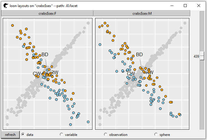
Figure 2: non-interactive layer
When the tour changes, this static layer does not change correspondingly (in GIF 6). To make it interactive, we have to create the following S3 function, by setting its class as background. The parameters of this function are
target: al_tourobject.layer: a layer to be turned into interactive.-
...includes that:start: the start matrix of projection vectors \(\boldsymbol{P}_s\)
initialTour: the activated panel’s initial position \(\boldsymbol{Y}_s\) where \(\boldsymbol{Y}_s = \boldsymbol{X} \boldsymbol{P}_s\).
projections: A list of the activated panel’s projection matrices.
tours: A list of the activated panel’s tour path (\(\boldsymbol{Y}\)).
group: a factor defines the grouping of the activated panel.
var: scroll bar current variable.
varOld: scroll bar previous variable.
color: the activated panel’s objects’ (points’ or lines’) color.
axes: only for scatterplot, the guided axes.
labels: only for scatterplot, the guided labels.
axesLength: only for scatterplot, the guided axes length.
-
If the layer is added for a
l_tour_compoundobjectl_compound: a
l_compoundwidgetallTours: returns the tour path for all panels.
allInitialTour: returns the initial position for all panels.
allProjections: returns the projection matrices for all panels.
allColor: returns the color for all panels
Notice that, there is no need to use all these to build an interactive statistical layer. For example, in function
l_layer_callback.background, we only extract two parametersallTours(the tours for all panels) andvar(the current scroll bar variable).
l_layer_callback.background <- function(target, layer, ...) {

  widget <- l_getPlots(target)
  layer <- loon::l_create_handle(c(widget, layer))

  args <- list(...)
  # the overall tour paths
  allTours <- args$allTours
  # the scale bar variable
  var <- args$var
  # the current projection (bind both facets)
  proj <- do.call(rbind, allTours[[var]])

  loon::l_configure(layer,
                    x = proj[, 1],
                    y = proj[, 2])
}
GIF 7: interactive layer
After function l_layer_callback.background is created and executed, the layer is interactive.