The loon package is designed for interactive data exploration. After exploring the events of interest, we need a tool to turn the interactive plots to static ones for publication. Snapshots of interactive loon plots can be captured in several ways:

via a screen shot of the window using <CTRL-P> (a primitive rendering of the plot saved as a file)
via a screen shot of the window from the host operating system (producing a file of several possible types), or
using plot() or loonGrob() to translate the plot to a grid graphic.

Of these, the last will be most convenient to incorporate plots in RMarkdown or to export them using some R environments (e.g., RStudio). This is the method discussed here.

By translating an interactive loon widget into a grid object, one can also later edit it to change or add fine details that otherwise might not be easily produced interactively.

See also the vignette “Saving loon plots”

Other packages within the diveR package suite are the loon.ggplot package and the loon.shiny package. These can be used to create elegant ggplot2 plots from loon plots (and incorporate into into RMArkdown documents) and to incorporate interactive loon plots for a curated exploratory analysis within in a shiny app.

Producing static `grid` plots

The grid graphics package is one of the fundamental graphics systems in R. It provides a low-level, general purpose graphics system for producing a wide variety of plots. Many well-known graphical systems, e.g. lattice and ggplot2, use grid to draw plots.

Here loon plots are transformed into grid graphics plots to provide, as close to possible, a wysiwyg snapshot of the interactive plot. Being grid graphics plots, these in turn can be edited using various grid functions.

Begin with a classic data set in R – mtcars which contains 32 automobiles and 11 (numeric) variables.

library(loon)
p <- with(mtcars, l_plot(mpg, hp, 
                         size = 8,
                         showScales = TRUE))

Here, p is a loon widget. The aesthetics attributes can be accessed either by function l_cget() or a simple [, as in

# x coordinates
p['x']

## [1] 21.0 21.0 22.8 21.4 18.7 18.1 14.3 24.4 22.8 19.2 17.8 16.4 17.3
## [14] 15.2 10.4 10.4 14.7 32.4 30.4 33.9 21.5 15.5 15.2 13.3 19.2 27.3
## [27] 26.0 30.4 15.8 19.7 15.0 21.4

# point size
p['size']

## [1] 8 8 8 8 8 8 8 8 8 8 8 8 8 8 8 8 8 8 8 8 8 8 8 8 8 8 8 8 8 8 8 8

These returned values always reflect the current states of p. For example, suppose the size of points is modified to 6 by direct manipulations on the plot, call p['size'], a length 32 vector of 6 is returned. With this handy “querying tool”, all essential elements of a loon widget can be accessed to construct a selfsame grid graphics, as in

# `p` is a loon widget
plot(p)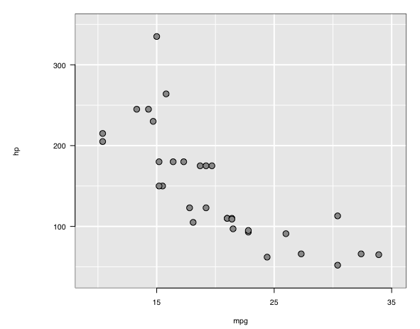

which produced and printed the plot p (as it presently appears) by first translating the loon plot into a grid graphics object (or grob). This can be used at any time, including in an RMarkdown document (as it is here).

For most users, no more need be done. This vignette could end here.
These users might also be interested in turning loon plots into ggplots (and vice versa); if so, some information on this is provided towards the end of this vignette in the ggplots section.

For those interested in a deeper understanding of the grid plots, read on.

Note: The plot() function is simply a wrapper function around the workhorse function loonGrob() which does the translatation from current display of the loon plot to a grid object (or grob) capturing the features of the loon display. The resulting grob is drawn using grid.draw() from the grid package.

`loonGrob()`: `loon` –> `grid` object

The grid graphic plot is saved by assigning it to a variable when it is created. Either drawing it at the same time (as a side-effect)

g0 <- plot(p)

or postponing the drawing to later as in

g0 <- plot(p, draw = FALSE)

Either way, a grid data structure is created and assigned to the variable g0.

Alternatively, loonGrob() can be called directly, as in

g0 <- loonGrob(p)

This returns a grid graphics object or grob. It can be drawn at any time using grid.draw() from the grid package.

library(grid)
grid.newpage()
grid.draw(g0)

multiple plots

As with any grob, the output of loonGrob()ccan be manipulated as can grid data structure – perhaps arranging several of these into a compound display using grid.arrange() (from the gridExtra package).

For example, there might be several stages of the interactive plot that ow might be captured. These might be constructed programmatically as

oldColor <- p["color"]
set.seed(3141)
selection <- sample(c(TRUE, FALSE), 
                    size = length(oldColor), 
                    replace = TRUE)
p["color"]  <- selection
gtrans <- loonGrob(p)
p["active"] <- selection
gauto <- loonGrob(p)
p["active"] <- !selection
gmanual <- loonGrob(p)
p["active"] <- TRUE
p["color"] <- oldColor

and then drawn in a single display

library(gridExtra)
grid.newpage()
grid.arrange(g0, gtrans, gauto, gmanual, nrow = 2)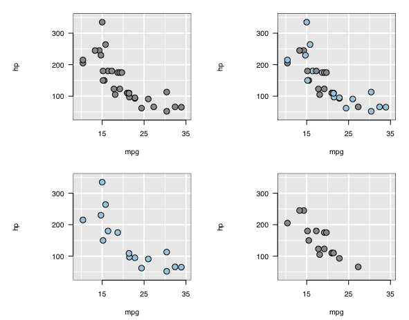

The arrangement itself could have been positioned within another arrrangement.

the data structure returned by `loonGrob()`

The returned data structure has

class(g0)

## [1] "gTree" "grob"  "gDesc"

This gTree object is a tree data structure in grid and contains the many grobs needed to draw the plot on demand. Numerous functions exist within the grid package for validating, drawing, and modifying grid graphical objects like this gTree and many of its elements.

The tree structure of g0 is easily seen using grid.ls() to list the contents:

grid.ls(g0)

## GRID.gTree.2
##   l_plot
##     bounding box
##     loon plot
##       guides
##         guides background
##         guidelines: xaxis (major), x = 15
##         guidelines: xaxis (major), x = 25
##         guidelines: xaxis (major), x = 35
##         guidelines: xaxis (minor), x = 10
##         guidelines: xaxis (minor), x = 20
##         guidelines: xaxis (minor), x = 30
##         guidelines: yaxis (major), y = 100
##         guidelines: yaxis (major), y = 200
##         guidelines: yaxis (major), y = 300
##         guidelines: yaxis (minor), y = 50
##         guidelines: yaxis (minor), y = 150
##         guidelines: yaxis (minor), y = 250
##         guidelines: yaxis (minor), y = 350
##       labels
##         x label
##         y label
##         title: textGrob arguments
##       axes
##         x axis
##           major
##           ticks
##           labels
##         y axis
##           major
##           ticks
##           labels
##       clipping region
##       l_plot_layers
##         scatterplot
##           points: primitive glyphs
##       boundary rectangle

The levels are indicated by indenting.

The following figure renders the tree structure more generally: 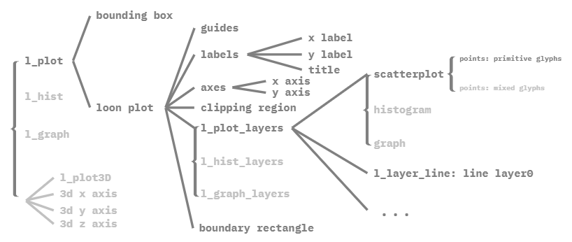Node labels give the loonGrob names with the tree hierarchy following solid lines from left to right. Grey values indicate the same for other types of loon plots (separate with braces) and identify potential options peculiar to each loon plot.

For example, the root node “l_plot” contains a “bounding box” and a “loon plot”, each loon plot has “guides”, “labels”, “axes”, “clipping region”, “boundary rectangle” and “l_xxxx_layers” (according to the type of loon plot), and the loon plot p has “l_plot_layers” consisting of a “scatterplot” and possibly other layers like lines and so on.

changing a `grid` object: get, edit, set

Knowing the labels, one can retrieve, edit, or even replace any fine details of the static plot. For example, consider the “xlabel” and “ylabel” of the gTree. Each label (as it appears above in the list of the gTree) provides a path to the corresponding grob.

Changes to an existing grid plot are made in three steps:

getGrob() to get a copy of the grob to be changed
editGrob() to produce a grob with the desired changes, and
setGrob() to set the newly produced grob into the appropriate place in the plot.

Each of these are now illustrated in turn.

`getGrob()`

Knowing the path is “x label” in the gTree g0, the grob is extracted using getGrob(). For example,

# retrieve xlabel grob
xlabelGrob <- getGrob(g0, "x label")
xlabelGrob

## text[x label]

class(xlabelGrob)

## [1] "text"  "grob"  "gDesc"

which itself has structure:

names(xlabelGrob)

##  [1] "label"         "x"             "y"             "just"         
##  [5] "hjust"         "vjust"         "rot"           "check.overlap"
##  [9] "name"          "gp"            "vp"

xlabelGrob$label

## [1] "mpg"

Note that xlabelGrob is a copy of the grob found at the “x label” path in g0.

Similarly grobs at other paths (e.g., “y label”) could be extracted and copied.

Note also that some elements of the gTree appearing in the listing grid.ls(g0) are actually parts of a grob and not the path itself. For example, consider the x-axis elements:

xAxisGrob <- getGrob(g0, "x axis")
names(xAxisGrob)

## [1] "major"  "ticks"  "labels"

names(xAxisGrob$children)

## [1] "at"            "label"         "main"          "edits"        
## [5] "name"          "gp"            "vp"            "children"     
## [9] "childrenOrder"

`editGrob()`

Having xlabelGrob in hand, we can use it to create another copy of it with changed features using editGrob().

For example, a more meaningful x axis “label” name can be assigned:

newGrob = editGrob(xlabelGrob, 
                   label = "Miles per (US) gallon")

The newGrob is now a textGrob

class(newGrob)

## [1] "text"  "grob"  "gDesc"

with the more informative label:

newGrob$label

## [1] "Miles per (US) gallon"

`setGrob()`

To complete the change to g0, the old “x label” needs to be replaced by newGrob:

g0 <- setGrob(gTree = g0, 
              gPath = "x label",
              newGrob = newGrob)

Now “xlabel” has been changed to “Miles/(US) gallon” within the grid plot g0.

grid.newpage()
grid.draw(g0)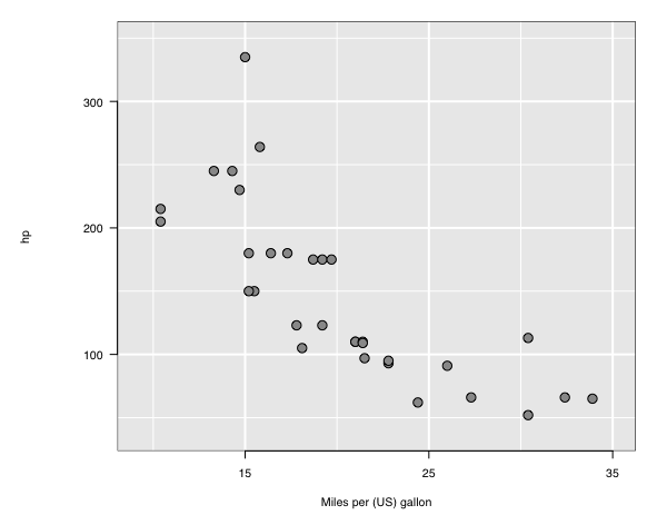

In the same way, other features of the “x label” could have been changed as well as the grobs at other paths of the gTree returned by loonGrob().

adding an alpha channel to the points

A more common place reason to edit would be to add features to the grid plot that are available in loon.

For example, transparency is (presently) missing from tcltk colours (on which loon is based) – the tcltk system presently uses 12 digit hexadecimal colour to represent three channels (one for each of the RGB colours) and no fourth channel indicating alpha transparency. In contrast, transparency is accommodated in grid graphics so that one might choose to set the alpha values after the transformation.

The points in the plot can be made transparent using setGrob(), editGrob(), and getGrob(), given the path to the points grob, namely “points: primitive glyphs”.

pathGrob <- "points: primitive glyphs"
newLoonPointsGrob <- 
  editGrob(
    getGrob(g0, pathGrob), 
    gp = gpar(fill = as_hex6color(p['color']),
              col = l_getOption("foreground"),
              fontsize = 20, # give a larger point size,
              alpha = 0.3 # turn color transparent
              )
    )
# update loon points grob
g0 <- setGrob(
  gTree = g0,
  gPath = "points: primitive glyphs",
  newGrob = newLoonPointsGrob
)
grid.newpage()
grid.draw(g0)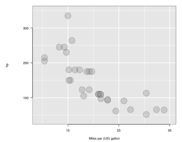

After modification, the points are now transparent and the size has been made larger.

helper functions from `loon`

Three loon helper functions simplify the some editing of the gTree produced by loon in the special case when some grobs on the gTree are incompletely specified.

The three helper functions are

l_instantiateGrob() which instatiates a complete grob using the information available on the incomplete description of the grob;
l_setGrobPlotView() which resets the margins of the grid plot to those of a loon plot when all labels and scales are shown (or to margin sizes specified in arguments); and
l_updateGrob() which behaves much like editGrob() except that it can work with incomplete grob descriptions and is called by l_instantiateGrob().

See help("loonGrobInstantiation") for more.

Common cases where these functions might be used are when pieces of the plot have been rendered invisible.

e.g. missing title

The plot p was not given a title and no title appears when g0 is drawn. Nevertheless, the gTree of g0 does appear to have some title information as indicated by the path “title: textGrob arguments”. This is an indication that loonGrob() did transfer some title information from p to g0 but that it is incomplete in some way.

If we access the grob at that path, we have

titleGrob <- getGrob(g0, "title: textGrob arguments")
titleGrob$label

## [1] ""

which has an empty label string and, looking at its class:

class(titleGrob)

## [1] "grob"  "gDesc"

appears not to be a text grob. Instead, it is an incomplete description, gDesc, of the grob.

g1 <- l_instantiateGrob(g0, "title: textGrob arguments",
                        label = "1974 Motor Trend cars data",
                        gp = gpar(col = "blue",
                                  fontsize = 8))
grid.newpage()
grid.draw(g1)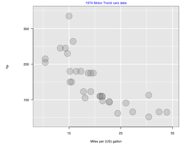

Note that the fontsize was chosen to be small so that it fit in the space available.

There was too little room for a standard title because the margins of the loon plot p were smaller with no title. An alternative to making the font small is to return the loon (or alternatively some user specified) margins to the plot using l_setGrobPlotView():

g2 <- l_instantiateGrob(g0, "title: textGrob arguments",
                        label = "1974 Motor Trend cars data",
                        gp = gpar(col = "red"))
g2 <- l_setGrobPlotView(g2)
grid.newpage()
grid.draw(g2)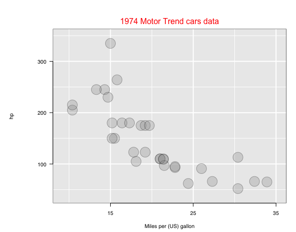

which displays the title in the default fontsize (from translating p). The extra room for the title would also admit larger font sizes.

e.g. missing labels

Oftentimes all labels (i.e., “xlabel”, “ylabel”, and “title”) of p will have been turned off when loonGrob() was called:

p['showLabels'] <- FALSE
g3 <- loonGrob(p)
grid.newpage()
grid.draw(g3)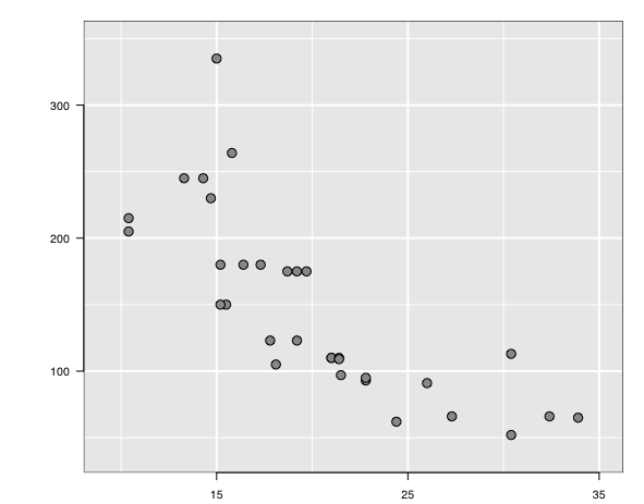

and we would like to turn these labels on in the static plot.

The gTree g3 now has a different path at each label.

grid.ls(g3)

## GRID.gTree.5
##   l_plot
##     bounding box
##     loon plot
##       guides
##         guides background
##         guidelines: xaxis (major), x = 15
##         guidelines: xaxis (major), x = 25
##         guidelines: xaxis (major), x = 35
##         guidelines: xaxis (minor), x = 10
##         guidelines: xaxis (minor), x = 20
##         guidelines: xaxis (minor), x = 30
##         guidelines: yaxis (major), y = 100
##         guidelines: yaxis (major), y = 200
##         guidelines: yaxis (major), y = 300
##         guidelines: yaxis (minor), y = 50
##         guidelines: yaxis (minor), y = 150
##         guidelines: yaxis (minor), y = 250
##         guidelines: yaxis (minor), y = 350
##       labels
##         x label: textGrob arguments
##         y label: textGrob arguments
##         title: textGrob arguments
##       axes
##         x axis
##           major
##           ticks
##           labels
##         y axis
##           major
##           ticks
##           labels
##       clipping region
##       l_plot_layers
##         scatterplot
##           points: primitive glyphs
##       boundary rectangle

Knowing the paths of the missing labels, the two helper functions (together with the desiredtextGrob() arguments) will construct the desired plot:

g4 <-l_instantiateGrob(g3, 
                       "title: textGrob arguments",
                       x = unit(8, "native"),
                       just = "left",
                       label = "Motor Trend Magazine 1974")

g4 <-l_instantiateGrob(g4, 
                       "x label: textGrob arguments",
                       label = "Miles per US gallon",
                       x = unit(35, "native"),
                       y = unit(-1.5, "lines"),
                       just = "right",
                       gp = gpar(fontsize = 15, 
                                 fontface = "italic",
                                 col = "blue"))

g4 <-l_instantiateGrob(g4, 
                       "y label: textGrob arguments",
                       label = "Horse power",
                       rot = 45,
                       x = unit(7, "native"),
                       y = unit(275, "native"),
                       just = "right",
                       gp = gpar(fontsize = 15, 
                                 fontface = "italic",
                                 col = "blue"))

g4 <- l_setGrobPlotView(g4)
grid.newpage()
grid.draw(g4)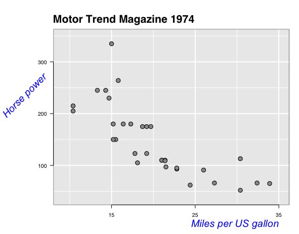

Extra arguments to l_instantiateGrob() are passed on to the grobFun (in this case textGrob()).

`l_updateGrob()`

This function is called by l_instantiateGrob() to perform the same role as editGrob(), but operating on incomplete grobs that are only gDescs.

The function l_updateGrob() could also be used the same as editGrob() on a complete grob (e.g. having classes text, grob, and gDesc).

What if …

some points are invisible?

Unfortunately, if some points are invisible, their coordinates and aesthetics attributes would be missing in the loonGrob. Technically speaking, it is possible to include these invisible points inside the loonGrob, however, what stops us doing so is that the data structure would have to be changed – a pointsGrob would have to be replaced by a gTree with several children pointsGrobs to preserve display order and distinguish visible from invisible point.

This solution seems overly complicated and so was not implemented. Better to simply make the changes interactively on the loon plot and then translate it again to a new grid data structure.

some points are not primitive glyphs?

loon provides non-primitive glyphs, e.g. text glyphs, image glyphs, polygon glyphs, et cetera. Once a non-primitive glyph is drawn, the grob label beneath scatterplot would be points: mixed glyph.

# add text glyph
carNames <- l_glyph_add_text(p, text = rownames(mtcars))
p['glyph'] <- carNames
# loonGrob
g2 <- loonGrob(p)
getGrob(g2, "points: mixed glyphs")

It returns a gTree object and each child is a textGrob.

grid.newpage()
grid.draw(g2)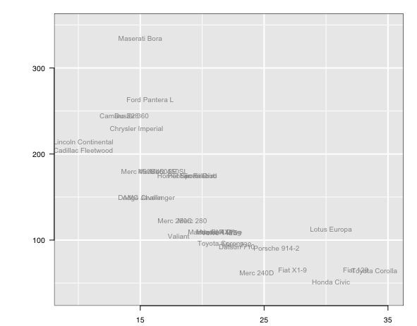

Other packages

`ggplot`s from `loon.ggplot`

Elegant print graphics are also provided through the popular ggplot2 package built on top of grid graphics. Users familiar with ggplot2 and its grammar of graphics might be interested in the loon companion package loon.ggplot which extends the grammar to a grammar of interactive graphics.

There any loon plot can be captured as a ggplot by simply calling loon.ggplot() on it. The same function will also create an interactive loon plot if called on an existing ggplot.

Details can be found here.

This is probably the simplest solution to have a static plot which can subsequently edited programmatically (via the grammar of ggplot2). Any changes to the ggplot could also then ve turned into an interactive loon plot.

`shiny` applications from `loon.shiny`

In the interest of supporting reproducible research, analysts will sometimes want to share interactive (and linked) plots in their curated analysis. A shiny app is the way to shared this interaction.

The loon companion package loon.shiny makes it possible to do just that by incorporating interactive loon style plots into a shiny app. Then the viewer may interactively explore the data under analysis inside an hyml browser. The interaction will not be as open ended as using loon in R but will be peculiar to the data in the app and to the features selected y the author.

The loon.shiny transformation relies on the loon to grid functionality described above. Details can be found here.

Loon plots and grid graphics

R. Wayne Oldford and Zehao Xu

September 17, 2021

Producing static `grid` plots

`loonGrob()`: `loon` –> `grid` object

multiple plots

the data structure returned by `loonGrob()`

changing a `grid` object: get, edit, set

`getGrob()`

`editGrob()`

`setGrob()`

adding an alpha channel to the points

helper functions from `loon`

e.g. missing title

e.g. missing labels

`l_updateGrob()`

What if …

some points are invisible?

some points are not primitive glyphs?

Other packages

`ggplot`s from `loon.ggplot`

`shiny` applications from `loon.shiny`

Loon plots and grid graphics

R. Wayne Oldford and Zehao Xu

September 17, 2021

Producing static grid plots

loonGrob(): loon –> grid object

multiple plots

the data structure returned by loonGrob()

changing a grid object: get, edit, set

getGrob()

editGrob()

setGrob()

adding an alpha channel to the points

helper functions from loon

e.g. missing title

e.g. missing labels

l_updateGrob()

What if …

some points are invisible?

some points are not primitive glyphs?

Other packages

ggplots from loon.ggplot

shiny applications from loon.shiny

Producing static `grid` plots

`loonGrob()`: `loon` –> `grid` object

the data structure returned by `loonGrob()`

changing a `grid` object: get, edit, set

`getGrob()`

`editGrob()`

`setGrob()`

helper functions from `loon`

`l_updateGrob()`

`ggplot`s from `loon.ggplot`

`shiny` applications from `loon.shiny`