Loon: An Interactive Statistical Visualization Toolkit

Scatterplot
Good To Know
Glyphs
- Primitive Glyphs
- Non-Primitive Glyph Types

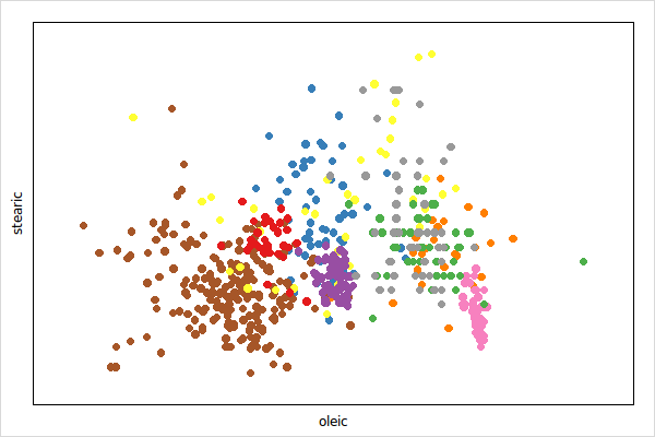
data(olive); attach(olive)
p <- l_plot(x=oleic, y=stearic, color=Area)

Scatterplot

Get the state names with

states <- l_info_states(p)
names(states)

Query a state, say background, as follows
```
p['background']
```
Change a state, say again background and foreground, as follows
```
p['background'] <- 'gray20'
p['foreground'] <- 'gray90'
```
alternatively, and more efficient if you modify more than one state, use
```
l_configure(p, background='gray20', foreground='gray90')
```

When creating a plot you may specify any state at plot creation

p1 <- l_plot(x=oleic, y=stearic, color=Area,
    background='gray20', foreground='gray90')

details on a state, say background, is easily had with
```
states <- l_info_states(p)
states$background
```
and a particular field
```
states$background$description
```

Good To Know

The scatterplot display supports layers.

Glyphs

The visual representation of a point can be changed for each point separately with the n dimensional state glyph. The supported glyph types are detailed in the following sections. The l_glyphs demo demonstrates all the glyph types.

Primitive Glyphs

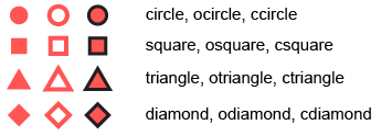
The supported primitives are circle, ocircle, ccircle, square, osquare, csquare, triangle, otriangle, ctriangle, diamond, odiamond and cdiamont.

data(olive); attach(olive)
p <- l_plot(x=oleic, y=stearic, color=Area)

glyphmap <- list(
    'South-Apulia'='circle',
    'North-Apulia'='ocircle',
    'Inland-Sardinia'='square',
    'Coast-Sardinia'='osquare',
    'East-Liguria'='triangle',
    'West-Liguria'='otriangle',
    'Calabria'='diamond',
    'Sicily'='odiamond',
    'Umbria'='cdiamond')

p['glyph'] <- unlist(glyphmap[as.character(Area)])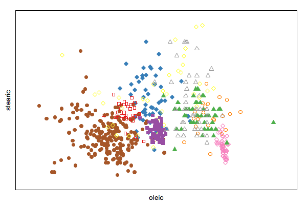

Non-Primitive Glyph Types

The non-primitive glyphs are the following

The non-primitive glyphs require user specified data. Adding a glyph type requires to specify the glyph data for each of the n points. If n of the plot changes the glyph will be deleted.

Glyphs, like plots and layers, have states and support state bindings. You can query and modify the glyph states, or add state bindings to glyphs at run time as shown below.

Text

Text glyphs are character strings for each point

gt <- l_glyph_add_text(p, text=as.character(Region))
p['glyph'] <- gt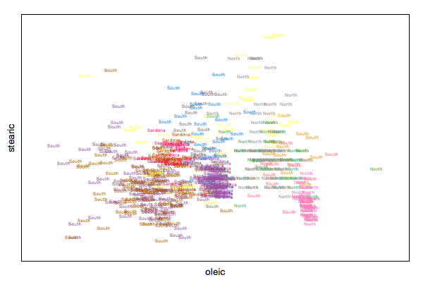

Serialaxes

Serialaxes glyph show either a star or a parralel coordinate glyph for each point.

gs <- l_glyph_add_serialaxes(p, data=olive[,-c(1,2)], showArea=FALSE)
p['glyph'] <- gs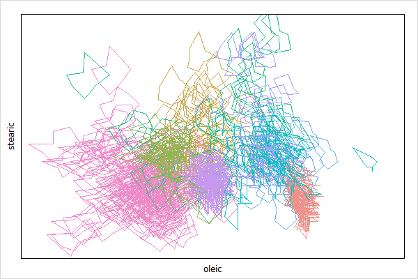

Change the glyph appearance as explained in Query and Modify Glyph States

l_configure(gs, axesLayout='parallel', showEnclosing=TRUE, showAxes=TRUE)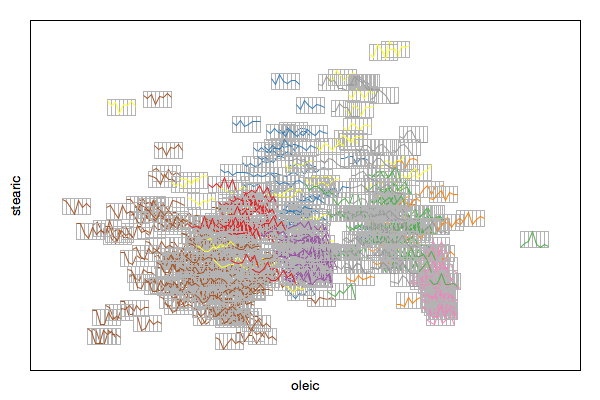

Please also see the serialaxes display documentation for more information regarding working with serialaxes.

Pointranges

If every point has a point range associated you can visualize this information with the pointrage glyph.

p1 <- l_plot(x=1:3, y=1:3, color=1:3)
gr <- l_glyph_add_pointrange(p1, ymin=c(0,1.5, 2.3),
    ymax=c(1.6,2.4,3.1), linewidth=1:3, showArea=FALSE)
p1['glyph'] <- gr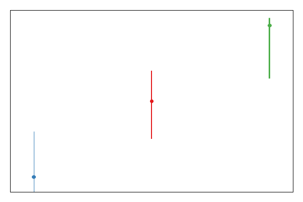

Polygons

A polygon can be a useful point glyph to visualize arbitrary shapes such as airplanes, animals and shapes that are not available in the primitive glyph types (e.g. cross). The l_glyphs demo has an example of polygon glyphs which we reuse here.

First we specify the coordinates of the polygons, note that it is your responsibility to center them at 0 and to specify an appropriate size. A good range for the polygon coordinates is from -1 to 1.

x_star <- 
    c(-0.000864304235090734, 0.292999135695765, 0.949870354364736, 
      0.474503025064823, 0.586862575626621, -0.000864304235090734, 
      -0.586430423509075, -0.474070872947277, -0.949438202247191,
      -0.29256698357822)
y_star <-
    c(-1, -0.403630077787381, -0.308556611927398, 0.153846153846154, 
      0.808556611927398, 0.499567847882455, 0.808556611927398,
      0.153846153846154, -0.308556611927398, -0.403630077787381)
x_cross <- 
    c(-0.258931143762604, -0.258931143762604, -0.950374531835206, 
      -0.950374531835206, -0.258931143762604, -0.258931143762604,
      0.259651397291847, 0.259651397291847, 0.948934024776722,
      0.948934024776722, 0.259651397291847, 0.259651397291847)
y_cross <-
    c(-0.950374531835206, -0.258931143762604, -0.258931143762604, 
      0.259651397291847, 0.259651397291847, 0.948934024776722,
      0.948934024776722, 0.259651397291847, 0.259651397291847,
      -0.258931143762604, -0.258931143762604, -0.950374531835206)
x_hexagon <-
    c(0.773552290406223, 0, -0.773552290406223, -0.773552290406223, 
      0, 0.773552290406223)
y_hexagon <- 
    c(0.446917314894843, 0.894194756554307, 0.446917314894843,
      -0.447637568424085, -0.892754249495822, -0.447637568424085)

Then you can use those polygon coordinates to specify polygon glyphs as follows

p <- l_plot(1:3, 1:3)

gl <- l_glyph_add_polygon(p, x = list(x_star, x_cross, x_hexagon),
                          y = list(y_star, y_cross, y_hexagon))

p['glyph'] <- gl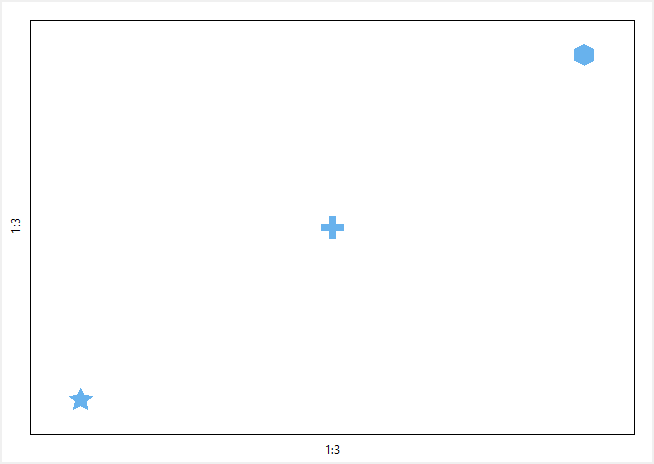

Images

Image glyphs rely on the Tcl procedure image_scale for image resizing. The loon package comes with a image_scale procedure that is pure Tcl code (i.e. interpreted). To improve the image resizing speed it is possible to install the ImageScale Tcl extension. loon will check when it is loaded whether the 'ImageScale' package is installed and will use the faster procedure (also in R).

We first start by creating the images manually and then show how to load images form files.

img1 <- as.character(tkimage.create('photo', width=30, height=20))
tcl(img1, 'put', 'blue', '-to', 0, 0, 30, 20)
tcl(img1, 'put', 'yellow', '-to', 0, 6, 30, 11)
img2 <- as.character(tkimage.create('photo', width=80, height=80))
tcl(img2, 'put', 'red', '-to', 0, 0, 80, 80)
tcl(img2, 'put', 'green', '-to', 30, 30, 60, 60)
img3 <- as.character(tkimage.create('photo', width=60, height=100))
tcl(img3, 'put', 'orange', '-to', 0, 0, 60, 100)
tcl(img3, 'put', 'black', '-to', 40, 0, 50, 80)

Note that the images above have different sizes. The loon scatterplot will resize the images (i.e. all glyph types) such that their areas are proportional to their associated point sizes.

The images are added as follows

p <- l_plot(x=c(1,2,3), y=c(3,1,2),
    color=c('green','yellow','blue'), size=c(4,3,7))

gi <- l_glyph_add_image(p, images=c(img1,img2,img3), label="Abstract Art")

p['glyph'] <- gi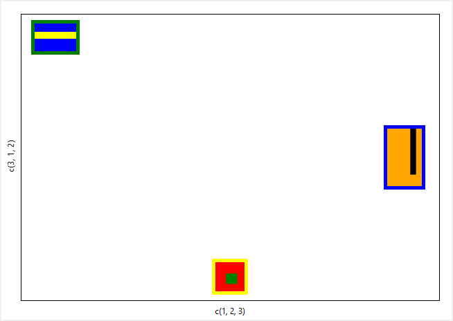

Load Images

Images must be in the standard tcl image format. Hence, you may read the image manual to get a deeper understanding of creating, deleting and querying images in tcl.

We do, however, provide two functions that simplify importing images from a set of files (jpg, png, bmp, etc.) and from an array with greyscale image information in its rows or columns, i.e. l_image_import_files and l_image_import_array, respectively.

If the images are stored in files in jpg, png or bmp format you can use our l_image_import_files function. The core tcl interpreter does not know many image formats but with tcl Img package loaded you can import images in the most common formats.

For the following example we use some images that we distribute with the loon R package

path <- system.file("images", package="loon")
image_paths <- dir(path, '*.png', full.names=TRUE)
imgs <- l_image_import_files(image_paths)

The tcl interpreter handles the image data internally and makes the image objects accessible via handles named image1, image2 and so on. The imgs object from above is hence a vector with the image object names. You can see the images in our image viewer as follows

l_imageviewer(imgs)

To add the images to a plot widget

p <- l_plot(1:length(imgs))

gi <- l_glyph_add_image(p, images=imgs, label="flags")

and to have the images displayed set the glyph plot state to the image glyphs

p['glyph'] <- gi

To see working examples, take look at one of the following loon package demos: l_ng_images_faces, l_ng_images_frey_LLE, or l_ng_images_frey_isomap. For example,

demo('l_ng_images_faces')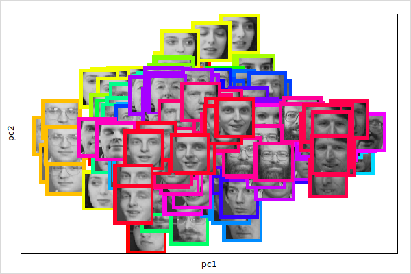

It is possible to fill pictures pixel by pixel or row by row as follows

library(tcltk); tt <- tktoplevel(); can <- tkcanvas(tt); tkpack(can)
pic <- tkimage.create('photo', width=20, height=30)
tkcreate(can, 'image', 50, 50, image=pic)
tcl(pic, 'put', 'yellow', '-to', 0, 0, 20, 30) # fill complete image
tcl(pic, 'put', 'red', '-to', 10, 15) # one pixel
# and row by row
.Tcl(paste(pic, 'put [list [lrepeat 16 blue] [lrepeat 16 green]] -to 0 17'))

Note that l_glyph_add_image creates copies of the submitted images. Hence, it is not possible to modify the images when the images are already on the canvas as it is the case in the above example.

Query and Modify Glyph States

The non-primitive glyphs (or n dimensional glyphs) have states. To demonstrate how to work with glyph states we take the text glyph example from above again:

data(olive); attach(olive)
p <- l_plot(x=oleic, y=stearic, color=Area)

gt <- l_glyph_add_text(p, text=as.character(Region))
p['glyph'] <- gt

The procedure to list and get information about them is similar as outlined in the states section. For example get the state names of a glyph with

gtstates <- l_info_states(gt)
names(gtstates)

Then to query a state, say text, use

gt['text']

And to modify a state

gt['text'] <- as.character(Area)

or, especially if you want to configure multiple states, you can use

l_configure(gt, text=as.character(Area))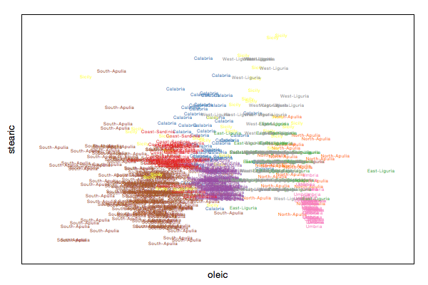

Relabel, List, and Deleting Glyphs

Glyph labels are used in the plot and glyph inspector. You can specify the glyph labels when creating the glyphs:

data(olive); attach(olive)
p <- l_plot(x=oleic, y=stearic, color=Area)

gt <- l_glyph_add_text(p, text=as.character(Region), label='Region')
p['glyph'] <- gt

or you may relabel once the glyphs already exist

l_glyph_relabel(p, id=gt, label='Region String')

Note, that the label is part of the glyph collection and not the glyph states.

To get all glyph ids with for a plot

l_glyph_ids(p)

To delete a glyph use

l_glyph_delete(p, id=gt)

When deleting a glyph every point that was displayed as that glyph will be switched to circle.

scatterplot - loon