It provides materials (i.e. serialaxes objects) to visualize high dimensional data in ggplot.

Documentation: https://great-northern-diver.github.io/ggmulti/

Introduction

Package ggmulti extends the ggplot2 package to provide some high dimensional visualization functionality, such as

• Serialaxes coordinates (i.e., parallel or radial axis systems)

• General glyphs (e.g., polygons, images) to appear a scatterplot.

• “More general” geom_histogram and geom_density to allow them to appear on serial axes.

Serialaxes Coordinates

Parallel coordinates

library(ggmulti)
p <- ggplot(iris, 
            mapping = aes(Sepal.Length = Sepal.Length,
                          Sepal.Width = Sepal.Width,
                          Petal.Length = Petal.Length,
                          Petal.Width = Petal.Width,
                          colour = Species)) +
       geom_path(alpha = 0.2) +
       coord_serialaxes()
p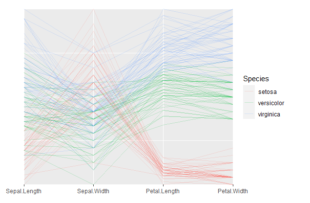

We can also construct a radar plot by setting axes.layout = "radial" in coord_serialaxes. In addition, we can add histogram layer on top

p + 
  geom_histogram(mapping = aes(fill = Species), alpha = 0.5)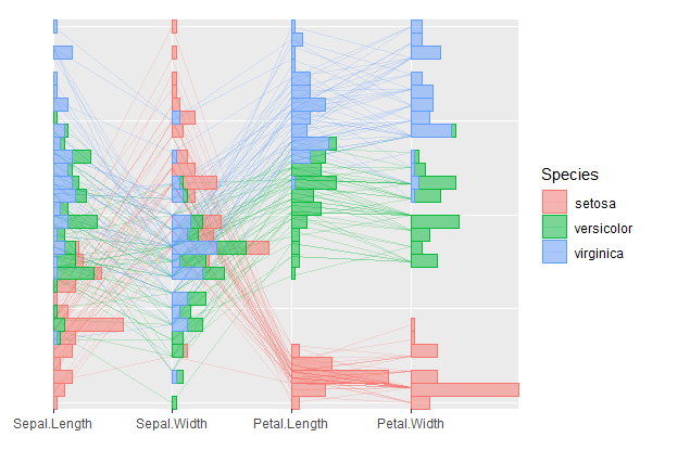

Glyphs

The flag of Canada

canada <- data.frame(
  xmin = c(-2, -1, 1),
  xmax = c(-1, 1, 2),
  ymin = rep(-1.2, 3),
  ymax = rep(1.2, 3),
  fill = factor(c(1,2,1))
)

p <- ggplot() + 
  geom_rect(data = canada, 
            mapping = aes(xmin = xmin, xmax = xmax, 
                          ymin = ymin, ymax = ymax,
                          fill = fill),
            colour = "black") + 
  geom_polygon_glyph(data = data.frame(x = 0, y = 0), 
                     mapping = aes(x = x, y = y),
                     polygon_x = x_maple,
                     polygon_y = y_maple, 
                     fill = "red",
                     size = 12) + 
  scale_fill_manual(values = c("red", "white")) + 
  theme_void() + 
  theme(legend.position = "none")
p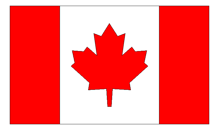

We can save it as a png object, then call geom_image_glyph to display the image glyph

ggsave("canada.png", type = "cairo", bg = "white")
images <- png::readPNG("canada.png")
ggplot(data = data.frame(x = c(1,2,1.5,2,1), y = c(1,1,1.5,2,2)),
       mapping = aes(x = x, y = y)) +
       geom_image_glyph(images = rep(list(images), 5)) + 
       coord_cartesian(xlim = extendrange(c(1,2)),
                       ylim = extendrange(c(1,2)))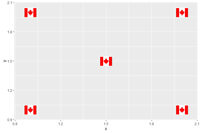

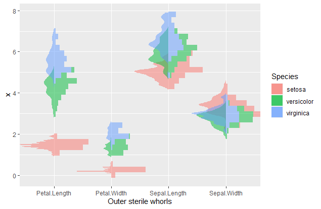
“More general” geom_histogram and geom_density

Functions geom_histogram_ and geom_density_ are more general geom_histogram and geom_density since these two functions can accommodate both x and y simutaniously. If only one is provided, geom_histogram or geom_density will be executed.

The following figure displays the back to back plot (histogram and density)

iris %>%
  tidyr::pivot_longer(cols = -Species,
                      names_to = "Outer sterile whorls",
                      values_to = "values") %>%
  ggplot(mapping = aes(x = `Outer sterile whorls`,
                       y = values, 
                       fill = Species)) +
  geom_histogram_(scale.y = "group",
                  alpha = 0.5,
                  prop = 0.6) + 
  geom_density_(scale.y = "group",
                prop = 0.6,
                alpha = 0.5,
                colour = NA,
                positive = FALSE)