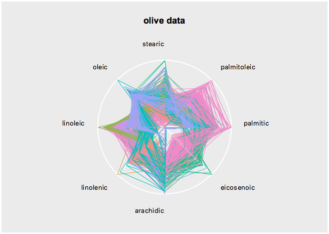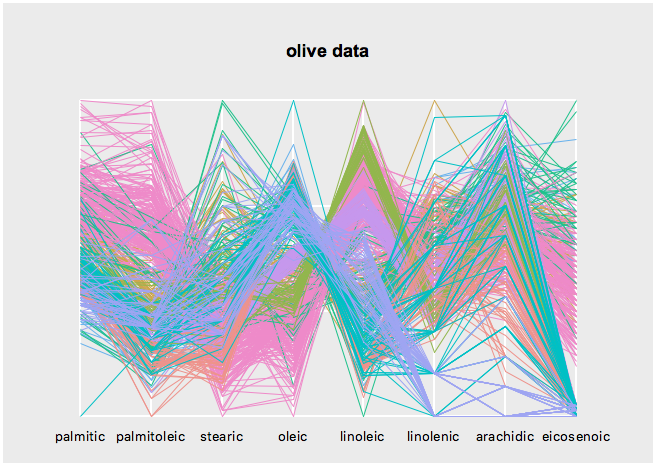
s <- l_serialaxes(data=oliveAcids, color=olive$Area, title="olive data")

s['axesLayout'] <- 'parallel'

Serialaxes

• Get the state names with

  states <- l_info_states(s)
  names(states)

• Query a state, say sequence, as follows

  s['sequence']

• Change a state, say again sequence, as follows

  s['sequence'] <- names(olive)[c(2:10)]

  alternatively, and more efficient if you modify more than one state, use

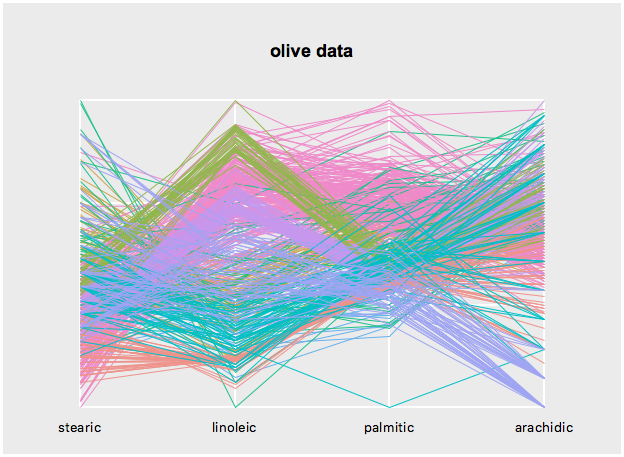
  l_configure(s, sequence=c('stearic', 'linoleic', 'palmitic', 'arachidic'))

  

• When creating a plot you may specify any state at plot creation

  s1 <- l_serialaxes(data=olive, color=olive$Area, title="olive data",
      sequence=names(olive)[2:10])

• details on a state, say sequence, is easily had with

  states <- l_info_states(s)
  states$sequence

  and a particular field

  states$sequence$description

Good To Know

• The serialaxes display does not support zooming and panning.
• Sweep selection is with a line and not with a rectangle.

Data Scaling

The scaling state defines how the data is scaled. The axes display 0 at one end and 1 at the other. For the following explanation assume that the data is in a nxp dimensional matrix. The scaling options are then

• variable: per column scaling.
• observation: per row scaling.
• data: whole matrix scaling.
• none: do not scale.