Loon: An Interactive Statistical Visualization Toolkit

Introduction

loon's displays that are based on Cartesian coordinates (i.e. scatterplot, histogram and graph display) allow for layering visual information including polygons, text and rectangles. Every layer has a unique id and the layer with the plot model (i.e. scatterplot points, histogram or graph) is called the model layer and has the id model.

The available layer types are the following

group: a layer that has no visual representation or states but can contain other layers
polygon: a single polygon
line: a single line with multiple segments
rectangle: a single rectangle
oval: a single oval
text: a single string

and n dimensional state or compound layers

points: n circles (with size state)
texts: n strings
polygons: n polygons
rectangles: n rectangles
lines: n lines

Note that for polygons, rectangles and lines the states x and y have a non-flat data structure , i.e. an R they use a list of vectors as follows

l_layer_polygons(p, x=list(c(1,2,3), c(4,2,1), c(1,2,3)),
    y=list(c(2,5,3), c(2,7,4), c(4,8,1)))

Some important implementation details for working with layers are

Currently only the model layer is interactive in the sense of selection and moving elements with mouse gestures.
Every layer has a unique id that is assigned by loon.
Layers are arranged in a tree structure where a group layer can be a parent to children layers (any of the above mentioned layer types). The tree root has id root.
The non-group layers are rendered in order of a Depth-first traversal of the layer tree.
Layers have states that define its appearance.
- Layer states support state bindings.
Sometimes (e.g. for texts layers), n can not be set to 1. Use the singular version instead (e.g. text).

To get a first impression on the possible operations that can be performed on layers you may query all commands that are available for working with layers

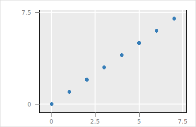
apropos("l_layer_")

Add, Move & Delete Layers

In this section we layer information onto the following scatterplot

p <- l_plot(x=0:7, y=0:7, showScales=TRUE, showGuides=TRUE,
    xlabel='', ylabel='')

The layer ids sub-command returns the plot's layer ids

l_layer_ids(p)

#> [1] "root"  "model"

The root and model layer exist in all plots. The root layer is the tree root and the model layer represents the visual representation of the data for the specific plot (e.g. histogram, scatterplot or graph).

The following code layers a polygon

l_p <- l_layer_polygon(p, x=c(0,1,2,3,3,2.5,1.5,0),
    y=c(5,4.5,4.5,5,7,7,5.5,5.2),
    color='black', linecolor='orange',
    linewidth=5)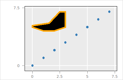

The variable l_p holds the layer id. In R the l_p has in addition a class and widget attribute. You can get the state descriptions as with normal plots

l_info_states(l_p)

Other layer types can be layered similarly, e.g.

l_l <- l_layer_line(p, x=c(0,2.5,5,7.5), y=c(4.5,0,6,3),
    linewidth=4, color='red')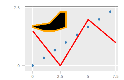

The layers are arranged in a tree structure and the rendering is according to the Depth-First algorithm of the visual layers in the tree. For example, we can layer a rectangle over the previous layers:

l_r <- l_layer_rectangle(p, x=c(0.5,6.5), y=c(0.5,6.5),
    color='green', linecolor='')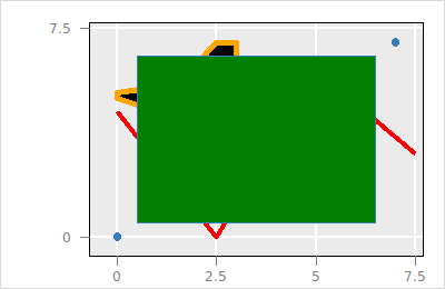

The rectangle with the layer id saved in the l_r variable over-plots the other layers, i.e. it is rendered last. To get a printout of the tree structure run

l_layer_printTree(p)

#> layer2
#> layer1
#> layer0
#> model

Hence the topmost layer, i.e. layer2, is rendered last. Layers can be moved with the l_layer_move function as follows

l_layer_move(p, layer=l_r, parent='root', index='end')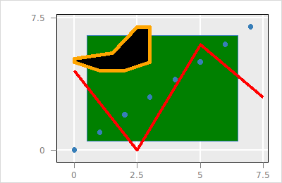

Note, that the parent layer, the index specifying the location among the parents children layers, and the label of a layer can also be specified when adding a layer. However parent, index and label are not states of the layer, instead they are information for the layer collection.

The following code creates a group and moves the polygon layer and line layer into it

l_g <- l_layer_group(p, parent='root', index='end')
l_layer_move(p, layer=l_l, parent=l_g, index='end')
l_layer_move(p, layer=l_p, parent=l_g, index='end')
l_layer_printTree(p)

#> layer3
#> model
#> layer2
#> +layer3
#>   layer1
#>   layer0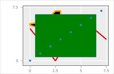

To move a layer one position up or down (i.e. change place with a sibling) one can also use the l_layer_raise and l_layer_lower function, respectively.

The visibility of a layer can be changed with the l_layer_hide and l_layer_show function.

l_layer_hide(p, l_g)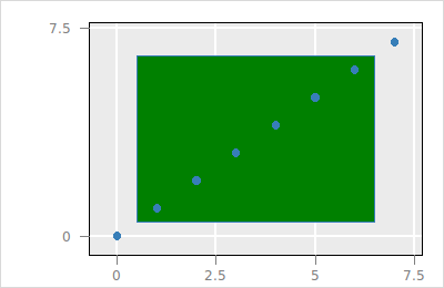

and

l_layer_show(p, l_g)

The layer with the rectangle can be deleted as follows

l_layer_delete(p, l_r)

If a group layer gets deleted with l_layer_delete then all its children layers get moved into their grandparent group layer. To delete a group layer and all it's children use the l_layer_expunge function.

l_layer_expunge(p, l_g)

It is also possible zoom and pan such that a particular layer fills the plot region

l_o <- l_layer_oval(p, x=c(2.5,5), y=c(2.5,5), color='thistle', index='end')
l_scaleto_layer(p, l_o)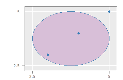

Query and Modify Layers

To modify the layer states works as described for plot states here. We start with the following histogram with a polygon layer:

h <- l_hist(x=c(1,1,2,1,4,3,2,2,1,4,5,4,3,2,4,3), binwidth=0.85,
    showScales=TRUE, showLabels=FALSE)

l_p <- l_layer_polygon(h, x=c(2,3,4,4.5,4,3.8,2.2),
    y=c(0.1,0,1,3,2,4,5), color='steelblue', linecolor='')

l_scaleto_world(h)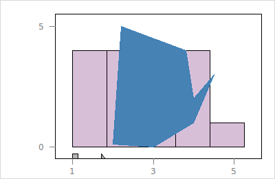

To query the state information use

l_info_states(l_p)

A layer state is queried as follows:

If l_p is of class l_layer
```
l_p['color']
```
or for multiple state changes
```
l_cget(l_p, 'color')
```
Or generally where l_p and h are only expected to be strings without a special class
```
l_cget(c(h, l_p), 'color')
```

A layer state is configured as follows:

If l_p is of class l_layer

l_p['color'] <- 'red'

or for multiple state changes

l_configure(l_p, color='red', linecolor='black')

Or generally where l_p is only expected to be a string without a special class
```
l_configure(c(h, l_p), linewidth=2)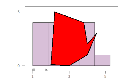
```

Maps

The loon R package also supports layering maps of classes defined in the sp and maps R packages. For a general overview of map data in R take a look at the CRAN Task View: Analysis of Spatial Data.

If you use the asSingleLayer=FALSE argument loon will create multiple individual polygon and line layers within a group. The default asSingleLayer=TRUE option will return a single polygons or lines layer. The default behavior is recommended as it keeps the displays faster.

maps library

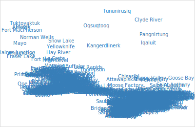
We start with maps in the maps. First we create a scatterplot with points located at the coordinates of Canadian citites

library(maps)
data(world.cities)

canada.cities <- subset(world.cities,
    grepl("canada", country.etc , ignore.case=TRUE))

p <- with(canada.cities,l_plot(x=long, y=lat, showLabels=FALSE))

g_t <- l_glyph_add_text(p, text=canada.cities$name)
p['glyph'] <- g_t

The canada regions are then layered as follows:

canada.map <- map("world",  "Canada", fill=TRUE, plot=FALSE)

id <- l_layer(p, canada.map,
    color = ifelse(grepl("lake", canada.map$names,
       ignore.case=TRUE), "lightblue", ""),
    asSingleLayer=FALSE)

l_scaleto_layer(p, id)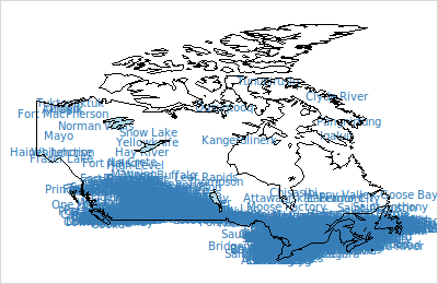

Note that if you would like every polygon to be an individual layer, you can use the asSinglelLayer=FALSE argument in the l_layer.map method.

sp library

Of the classes currently defined in the sp package for geographical data we currently support to layer of class Polygon, Polygons, SpatialPolygons, and SpatialPolygonsDataFrame. There are a couple of sources that provide map data for R using these classes, see

This example uses data from the Global Administrative Areas. We start by layering an outline of Switzerland into a scatterplot with 0 points:

con <- url("http://biogeo.ucdavis.edu/data/gadm2/R/CHE_adm0.RData")
load(con)
close(con)
    
p <- l_plot()
g <- l_layer_group(p, label="Switzerland")
m <- l_layer(p, gadm, label="Switzerland", parent=g,
             asSingleLayer=FALSE,
             color="", linecolor="black")
l_scaleto_world(p)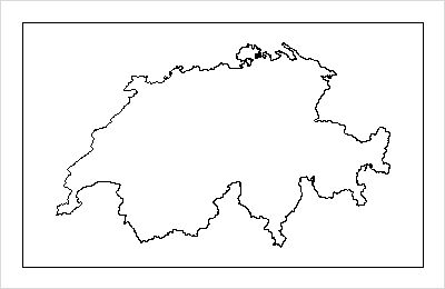

We continue by layering the outlines for the Swiss Cantons:

l_layer_hide(p, g)

g1 <- l_layer_group(p, label="Swiss Cantons")

con <- url("http://biogeo.ucdavis.edu/data/gadm2/R/CHE_adm1.RData")
load(con)
close(con)

m1 <- l_layer(p, gadm, label="Swiss Cantons", parent=g1, index=1,
              asSingleLayer=FALSE,
              color="", linecolor="red")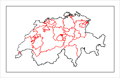

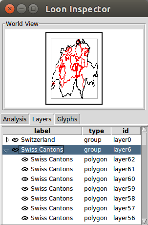
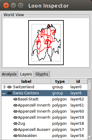
Finally, we label the canton layers accordingly

cantons <- gadm@data$NAME_1[gadm@plotOrder]

for (i in 1:length(m1)) {
    sapply(m1[[i]], function(l)l_layer_relabel(p, l, cantons[i]))
}

Generics

l_layer is a generic function and you may add a method to layer a visual representation for an object of a particular class.

methods('l_layer')

Here a short example for an object of class foo

newFoo <- function(x, y, ...) {
    r <- list(x=x, y=y, ...)
    class(r) <- 'foo'
    return(r)
}

Then the layer function is

l_layer.foo <- function(widget, x) {
    x$widget <- widget
    id <- do.call('l_layer_polygon', x)
    return(id)
}

And finally

p <- l_plot()

obj <- newFoo(x=c(1:6,6:2), y=c(3,1,0,0,1,3,3,5,6,6,5), color='yellow')

id <- l_layer(p, obj)

l_scaleto_world(p)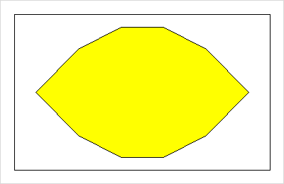

countourLines & heatImage & rasterImage

We provide the functions l_layer_contourLines, l_layer_heatImage, and l_layer_rasterImage that similar to the R functions contourLines, image, and rasterImage, respectively. See the examples for each function with the examples R function.

For example:

kest <- with(iris, MASS::kde2d(Sepal.Width,Sepal.Length))
p <- with(iris, l_plot(Sepal.Width,Sepal.Length, color='black'))
l_layer_contourLines(p, kest)
l_layer_heatImage(p, kest) 
l_scaleto_world(p)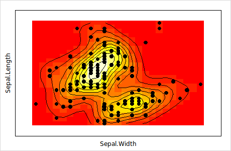

l_layer_contourLines creates a lines layer, and l_layer_heatImage, and l_layer_rasterImage a rectangles layer.

learn layering information - loon